Widespread Incorrect Implementation of the Hoffmann Method, the Correct Approach, and Modern Alternatives

Abstract

Objectives

The Hoffmann method is a procedure for reference interval estimation using routine clinical results. Many authors incorrectly prepare Hoffmann plots on a linear rather than normal probability scale. We explore the consequences.

Methods

This was investigated algebraically, by random number simulations (45 simulations, n = 100,000 each) and using clinical data sets. Strategies compared were: Hoffmann’s method as originally and incorrectly implemented, Bhattacharya’s method, and maximum likelihood (ML). All R source code and data sets are provided.

Results

As the proportion of healthy individuals approaches 1, the incorrect approach generates reference interval estimates of approximately μ_H ± 1.19 σ_H delineating the central 77% of the healthy subpopulation, not the central 95%. Inappropriately narrow reference interval estimates were seen on random simulations and clinical data sets. ML methods performed best.

Conclusions

The erroneous variant Hoffmann method should not be used. ML methods outperform others and are not restricted by Gaussian assumptions.

In 1963, Hoffmann described a simple graphical method for estimating reference intervals from routine laboratory data.¹ He assumed that the distribution of results could be represented by a mixture of two underlying Gaussian distributions, corresponding to the healthy and diseased subpopulations, with the healthy subpopulation dominating the sample Figure 1.

Figure 1

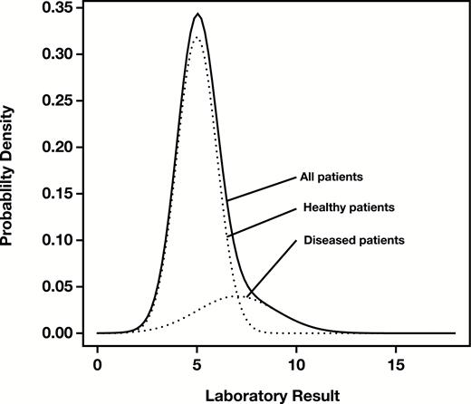
Density of a distribution of mock patient data for a hypothetical analyte consisting of a mixture of Gaussian distributions representing healthy (subscript H) patients (⁠${\mu }_H=5$⁠, ${\sigma }_H=1$⁠) and diseased (subscript D) patients (⁠${\mu }_D=7,$${\sigma }_D=2$⁠). Solid line, overall density; dotted lines, component densities.

Hoffmann’s method consisted of tallying the full set of results into a set of ordered categories representing measurement ranges (“bins”), calculating the cumulative frequencies of the categories and converting them to percentages, and using normal (Gaussian) probability paper to plot the cumulative percentages (on the y-axis with a Gaussian probability scale) against the measurement values corresponding to the category endpoints (on the x-axis with a linear scale).

Hoffmann demonstrated that under these assumptions, the result was a plot with two regions of approximate linearity corresponding to the healthy and diseased subpopulations. By extrapolating the linear region for the healthy individuals to the horizontal lines representing the 2.5th and 97.5th percentiles, the estimated reference interval corresponding to the central 95% of the healthy subpopulation could be read from the x-axis. Figure 2 illustrates the procedure for a set of $n=100$ simulated observations drawn from the theoretical density shown in Figure 1 where the procedure gives an estimated reference range of 3.0 to 7.3 compared to the actual reference range derived from simulation parameters of 3.0 to 7.0.

Figure 2

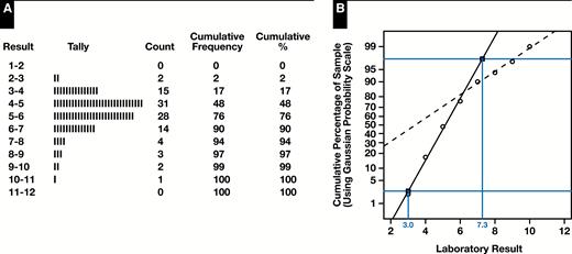
Original Hoffmann method applied to a simulated sample of $n=80$ healthy and $n=20$ diseased individuals from the mixture distribution shown in Figure 1. A, Tally of sample into a set of measurement ranges together with cumulative percentages. B, Hoffmann plot of right-midpoint of range (x-axis) vs cumulative percentage on Gaussian probability scale (y-axis), with extrapolated linear regions corresponding to healthy (solid line) and diseased (dashed line). Gray horizontal lines represent the 2.5th and 97.5th percentiles, and where those lines intersect the extrapolated “healthy” linear region, the x-coordinates give the estimated reference interval.

While “binning” the data made the traditional manual procedure more convenient, it is not a critical component of the approach. A correct modern approach involves sorting the $n$ measurements, assigning each measurement its corresponding cumulative probability (ie, assigning the $i$th ordered measurement the cumulative probability $i/n$ or using a similar formula with a small continuity correction), and plotting those probabilities (y-axis) against the measurement values (x-axis), thereby forming an empirical cumulative distribution function (CDF) of the sample. However, a critical component of the procedure is that the CDF be plotted using a Gaussian probability scale for the y-axis or, equivalently, that corresponding quantiles of a standard Gaussian distribution be plotted on a linear y-axis Figure 3. Such a plot is known as a “normal probability plot” and is a specific type of quantile-quantile (QQ) plot for which the comparator distribution is the standard Gaussian distribution.²

Figure 3

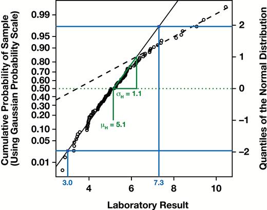
Correct modern variant of the Hoffmann method, plotting the measurement values (x-axis) against the cumulative probabilities of the sorted sample using a Gaussian probability scale (left y-axis) or equivalently against the corresponding quantiles of a standard Gaussian distribution (right y-axis). Extrapolation of the linear segment for the “healthy” linear region and estimation of the reference range may proceed as with the original method (blue), or by first estimating the mean and using the slope against the right (linear) y-axis to calculate ${\sigma }_H$ by ${\sigma }_H=1/slope$ (green).

The Hoffmann method has been widely applied in the field of clinical chemistry for reference interval derivation and reference interval validation.^3-22 There is also interest in automating the procedure.^14,15

Early papers describing or applying the method were true to the methodology as originally described by Hoffmann and clearly explained the purpose and necessity of using a Gaussian probability scale for the cumulative probabilities plotted on the y-axis.^23-25 Unfortunately, with only a few notable exceptions,^18,26,27 a host of modern papers^8,12-17,19 and even some textbooks¹¹ explicitly show the use of an incorrect method that involves plotting a CDF of the sample in purely linear space.

While it may seem inconsequential, this methodological deviation results in incorrect reference interval estimates in all circumstances, even in the ideal case of a single, unmixed Gaussian distribution representing measurements from only healthy individuals. Correspondingly, the parameter estimates of ${\mu }_H$ and ${\sigma }_H$ may be poor, the latter being generally (but not universally) too small, resulting in reference intervals much narrower than those generated by the correctly formulated Hoffmann method.

Although many approaches exist for Gaussian mixture model decomposition,²⁸ in clinical chemistry attention has been focused primarily on the strategies of Hoffmann and Bhattacharya,²⁹ likely because both are graphical in nature. The Bhattacharya method relies on first categorizing the measurements of laboratory quantity $x$⁠, into equally spaced classes (bins) of width $h$⁠. This results in frequencies, denoted $y,$ for each class. The quantity $\Delta log(y)=log(y(x+h))-log(y(x))$ is then plotted against x and, for appropriately chosen widths $h$⁠, the resulting plot will have regions where the curve straightens and has a negative slope. Extrapolation of these linear regions allows the determination of the x-intercept and the angle formed with the negative x-axis from which the mean, standard deviation, and proportion $p$ for each contributing mode can be calculated.²⁹ The method remains popular.³⁰

In contrast, a modern (nongraphical) computational strategy for this problem is the use of maximum likelihood (ML) through the expectation maximization algorithm.³¹ A description of how ML methods work is beyond the scope of this paper and the interested reader is directed to a review on the topic.²⁸ Importantly, however, the ML strategy for this and other problems has been implemented in relatively easy to use open-source computational packages for the R statistical programming language.

In what follows, we will demonstrate the magnitude of the error associated with the use of a linear CDF, both algebraically and with random number simulations. We will also compare different methods for parameter estimation: the Hoffmann method (both correctly and incorrectly implemented), the Bhattacharya method, and modern ML approaches using a select two^32,33 of several freely available software packages^32-36 implemented using the R statistical programming language, which can be applied to this and other related problems.

Materials and Methods

Using algebraic methods, we analyzed and compared the reference interval estimates generated by both a correct modern variant of the Hoffmann method and the commonly used but incorrect implementation using a linear CDF. We further characterized the theoretical behavior of estimates generated by each method in a number of extreme, but illustrative, cases: a single Gaussian distribution representing a population of healthy individuals only, and examples with both negligible and very large differences in healthy and diseased subpopulation means. We also described a typical illustrative case with a large healthy subpopulation and a small diseased subpopulation having modest separation between the subpopulation means.

We then compared approaches with random number simulations. Samples of size $n=100,000$ from two-component Gaussian mixture distributions were randomly generated to simulate a variety of situations: with ${\mu }_H=10$ and ${\mu }_H=1$ fixed, ${\mu }_D$ and ${\sigma }_D$ ranged from 12 to 18 and 1 to 3, respectively, and ${\rho }_H$ ranged from 0.7 to 0.9 (45 combinations in total). Each simulated sample was evaluated using multiple procedures to recover ${\mu }_H$⁠, ${\sigma }_H$⁠, the reference interval ${\mu }_H\pm 1.96{\sigma }_H$ and other parameters where applicable. The procedures employed were: a correct modern variant of the Hoffmann method, the incorrect Hoffmann variant, the Bhattacharya method, and a modern ML method from the R mixtools package.³³ Hoffmann and Bhattacharya linear sections were identified using visual oversight as prescribed. ML methods were provided crude starting parameter estimates of ${\mu }_H=11$⁠, ${\mu }_D=15$⁠, ${\sigma }_H=0.5$⁠, and ${\sigma }_D=1.5$ for all simulations. Procedures were evaluated for their performance in reproducing the correct results based on the known simulation parameters.

We also applied the procedures to deidentified, routine clinical laboratory datasets to illustrate performance differences between approaches. The datasets used included a hemoglobin (Hb) dataset with easily resolved and approximately Gaussian healthy and diseased subpopulations, a thyroid stimulating hormone (TSH) dataset with a highly skewed distribution and multiple (hyperthyroid and hypothyroid) diseased subpopulations, and a plasma calcium dataset with poor separation between the healthy and diseased subpopulations. Hb analyses were performed on a Sysmex XN-3000, TSH analyses were performed on a Roche Cobas e601, and calcium analyses were performed using the Arsenazo III method on the Siemens Advia 1800. All analyses were performed according to manufacturer specifications. Results for Hb, TSH, and calcium were extracted from laboratory information system from the entire 2016 calendar year. For clinical data, in addition to the parameter estimation methods applied to simulation data, the R mixdist³² package was employed because it permits the use of other distributions, including the gamma distribution which, depending on its so-called shape and rate parameter values, can both exhibit skewing and approximate the normal distribution.³⁷

This study was waived from ethics review by the research ethics boards of St Paul’s Hospital and the University of British Columbia as a quality initiative. All computational analyses were performed using R version 3.4.4 (supplemented with the dplyr, magrittr, mixtools, mixdist, and xtable R packages). Our work is an example of reproducible research,³⁸ and the Supplemental Data includes the article in the form of a literate program (including all text and source code in a single document) written using the rmarkdown package³⁹ (all supplemental data are available at American Journal of Clinical Pathology online).

Results

Algebraic Results

As shown in Supplemental Appendix 1, the correct modern variant of the Hoffmann method (as illustrated in Figure 3) will give estimated upper and lower limits of normal (LLN and ULN) approximated by the formula:

$$\begin{array}{c}\text{Correct Limits}\simeq {\mu }_H+\frac{A\times B}{\frac{1}{\sqrt{2\pi }}\frac{p_H}{{\sigma }_H}+\frac{p_D}{{\sigma }_D}\varphi (z_D)}\\ whereA=\left(\pm z_{\alpha /2}-{\Phi }^{-1}\left(\frac{1}{2}{p}_H+p_D\Phi (z_D)\right)\right)\\ B=\varphi \left({\Phi }^{-1}\left(\frac{1}{2}{p}_H+p_D\Phi (z_D)\right)\right)\end{array}$$

and where $\Phi (t)$ and $\varphi (t)$ are the CDF and probability density function, respectively, of a standard Gaussian distribution, $z_D=({\mu }_H-{\mu }_D)/{\sigma }_D$⁠, and $\alpha$ determines the size of the $(1-\alpha )\times 100\%$ normal range (eg, $\alpha =0.05$ for a 95% normal range).

In contrast, if the operator employs an incorrect variant of the Hoffmann method by plotting an empirical CDF in purely linear space and fitting a line to its apparently linear section, the resulting LLN and ULN will be given by the approximate formula:

$$\text{Incorrect normal limits}\simeq {\mu }_H+\frac{\frac{1}{2}\pm \frac{1-\alpha }{2}-\left(\frac{1}{2}{p}_H+p_D\Phi (z_D)\right)}{\frac{1}{\sqrt{2\pi }}\frac{p_H}{{\sigma }_H}+\frac{p_D}{{\sigma }_D}\varphi (z_D)}$$

While these results have a number of ramifications (Supplemental Appendix 1), the most striking pertains to the situation where the sample population is predominantly healthy, which is the usual context for use of indirect reference interval estimation methods.^40,41 Specifically, if $p_H$ is close to 1, then, as shown in Supplemental Appendix 1, the correct and incorrect LLN and ULN estimates (for $\alpha =0.05$⁠) will approach:

$$\begin{array}{cc}\hfill \text{Correct normal limits}& \begin{array}{c}\simeq {\mu }_H\pm z_{\alpha /2}{\sigma }_H\\ \approx {\mu }_H\pm 1.96{\sigma }_H\end{array}\\ \text{Incorrect normal limits}& \begin{array}{c}\simeq {\mu }_H\pm \sqrt{\pi /2}(1-\alpha ){\sigma }_H\\ \approx {\mu }_H\pm 1.19{\sigma }_H\end{array}\end{array}$$

This means that the reference intervals generated by the incorrect variation will be approximately 40% too narrow, with the LLN and ULN delineating the central 77% of the distribution rather than its central 95%. In contrast, the Hoffmann approach as originally described and its correct modern variant will produce LLN and ULN estimates that converge to ${\mu }_H\pm 1.96\sigma$ under these same circumstances. This finding is confirmed using random number simulations in Supplemental Appendix 1 along with a number of other illustrative examples.

Simulation Results

Supplemental Figures 1-9 show the results of 45 simulated scenarios (five scenarios per figure). Each is a sample of size $n=100,000$ simulated from a two-component Gaussian mixture with simulation parameters as summarized in Supplemental Table 1. For each simulation, the corresponding figure shows a histogram of the resulting mixture distribution and the application of the Bhattacharya method, a correct modern variant of the Hoffmann method, and the incorrect Hoffmann variant. The estimates of the means, standard deviations, and reference intervals (LLN and ULN) for these three graphical methods and modern ML methods, together with the error associated with each method, are shown in Supplemental Table 1.

The tendency of the incorrect variant of the Hoffmann method to produce reference intervals that are too narrow as $p_H\to 1$ is illustrated in Figure 4 and Supplemental Figure 1, Figure 4, and Figure 7 (where $p_H=0.9$⁠). The simulated example in Supplemental Appendix 1, Section A.4.1 illustrates the same phenomenon in the extreme case where $p_H=1.0$⁠, representing samples taken from an entirely healthy population.

Figure 4

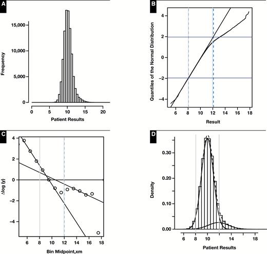
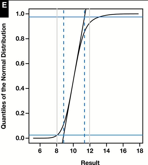
Results of representative random number simulation for which n = 100,000, ${\rho }_H=$ 0.9, ${\mu }_H=$ 10, ${\sigma }_H=$ 1, ${\mu }_D=$ 12, and ${\sigma }_D=$ 1.6. A, Histogram of mixture distribution. B, Hoffmann plot. Normal range estimate: 8.07 to 12.11. C, Bhattacharya plot. Normal range estimate: 8.05 to 11.99. D, Density plots of healthy and diseased modes (solid black lines) and their composite (dashed line) as determined by maximum likelihood (mixtools). Normal range estimate: 8.04 to 11.95. E, Incorrect approach to the Hoffmann method using a cumulative distribution function. Normal range estimate: 8.84 to 11.35. In all cases, vertical dashed lines represent method estimate of normal range and vertical gray lines represent ${\mu }_H\pm 1.96{\sigma }_H=$ 8.04 to 11.96.

Across the 45 random simulations, the median absolute errors of the estimates using the correct modern variant of the Hoffmann method were 2.2% for ${\mu }_H$ and 7.2% for ${\sigma }_H$⁠. In comparison, the errors for the widely used but incorrect variant using a CDF in linear space were 3.1% and 25%, respectively; errors for the Bhattacharya method were 0.5% and 9.9%; and errors for modern ML methods using the mixtools package were 0.0% and 0.3%. These results are demonstrated graphically in Figure 5.

Application to Real Laboratory Data

Results of applying these methods to real patient data—adult male outpatient Hb, adult TSH (inpatient and outpatient), and adult plasma calcium (inpatient and outpatient)—are shown in Table 1, with additional detail given in Supplemental Appendix 2. For ML analyses, TSH results greater than 15 mIU/L and calcium results below the 1st percentile and above the 99th percentile were removed prior to analysis to facilitate convergence.

Table 1

Results of Mixture Model to Clinical Data for Three Representative Scenarios: Well-Resolved Populations (Male Outpatient Hb), Skewed and Multimodal (Adult TSH), and Poorly Resolved (Total Calcium)

Analyte	Method	${\mu }_H$	${\sigma }_H$	${\mu }_D$	${\sigma }_D$	${\rho }_H$	LLN	ULN
Hb	Hoffmann-QQ	13.90	1.40	10.6	1.5		11.10	16.70
Hb	Bhattacharya	14.50	1.20	9.3	1.3	0.7	12.10	16.90
Hb	ML-mixtools	14.50	1.30	10.0	1.6	0.63	12.00	17.10
Hb	ML-mixdist	14.50	1.30	10.0	1.6	0.63	11.90	17.00
Hb	Hoffmann-CDF	13.50	1.30				11.00	16.10
TSH	Hoffmann-QQ	1.60	0.80				0.00	3.15
TSH	Bhattacharya	1.22	0.90				–0.54	2.98
TSH	ML-mixtools- normal	1.62	0.91	0.10, 4.85	0.08, 2.70	0.78	–0.15	3.40
TSH	ML-mixdist- gamma	1.98	1.31	0.07, 7.82	0.05, 2.86	0.92	0.29	5.25
TSH	Hoffmann-CDF	1.70	0.70				0.36	3.04
Ca	Hoffmann-QQ	9.10	0.70				7.80	10.35
Ca	Bhattacharya	9.13	0.60				7.96	10.30
Ca	ML-mixtools- normal	9.14	0.62	7.79	0.45	0.90	7.93	10.35
Ca	ML-mixdist- normal	9.15	0.62	7.79	0.45	0.90	7.94	10.35
Ca	ML-mixdist- gamma	9.21	0.58	8.00	0.53	0.83	8.12	10.38
Ca	Hoffmann-CDF	9.10	0.40				8.31	9.86

Ca, calcium; CDF, cumulative distribution function; Hb, hemoglobin; LLN, lower limit of normal; ML, maximum likelihood; QQ, quantile-quantile; TSH, thyroid stimulating hormone; ULN, upper limit of normal; μ_D, mean of the diseased population ; μ_H, mean of the healthy population; σ_D, standard deviation of the diseased population; _σH, standard deviation of the healthy population.

For the Hb and calcium datasets, where the reference interval estimation problem is more straightforward, the incorrect variant of Hoffmann’s method using a CDF in linear space produces narrower reference intervals and significantly different parameter estimates, compared to the other methods. For the TSH example, comparison of methods is complicated by the highly skewed distribution and the multiple diseased subpopulations (hypo- and hyperthyroidism). The distribution of TSH data does not satisfy the assumptions of the Hoffmann, Bhattacharya, or modern Gaussian-based ML methods, and all methods produce estimates that appear clinically incorrect, with ULN that seem too low. However, using modern ML methods with non-Gaussian model assumptions (a mixture of gamma distributions in this case), provides a superior fit and produces clinically plausible reference interval estimates (Supplemental Appendix 2).

Discussion

Random simulations illustrate a number of points. First, the normal QQ plot used in the correct implementation of the Hoffmann method is very sensitive to deviations from a Gaussian distribution. This has the effect of clearly resolving the linear segments corresponding to the healthy and diseased subpopulations and facilitates proper identification of the former. In contrast, the incorrect approach typically produces a sigmoidal shape in all situations, with no clear delineation of the healthy and diseased subgroups. The apparently linear region in the middle portion of the CDF does not necessarily correspond preferentially to the healthy subpopulation as the contributions of the two subpopulations tend to blend imperceptibly. Extension of this linear section has no particular meaning beyond identifying the steepest tangent line to the CDF, and the resultant parameter estimates are related in uninformative ways to the correct results. This effect can be appreciated by inspecting the progressions seen as ${\mu }_D$ approaches ${\mu }_H$ in the Supplemental Figures and in a representative simulation shown in Figure 4.

Second, while the Hoffmann method, when correctly implemented, is imperfect and will generally overestimate the ULN when ${\mu }_D>{\mu }_H$ (or, conversely, underestimate the LLN when ${\mu }_D<{\mu }_H$⁠), its estimates are fairly accurate provided $p_H\gtrsim 0.7$ as shown in Figure 5. Moreover, these biases tend to be both modest and predictable in nature. In contrast, with the incorrect variant of the method, the limits of the normal range may be underestimated or overestimated depending on the specifics of the proportions, means, and variances of the healthy and diseased modes (as illustrated in the Supplemental Figures, Supplemental Appendix 1, and Figure 5).

Figure 5

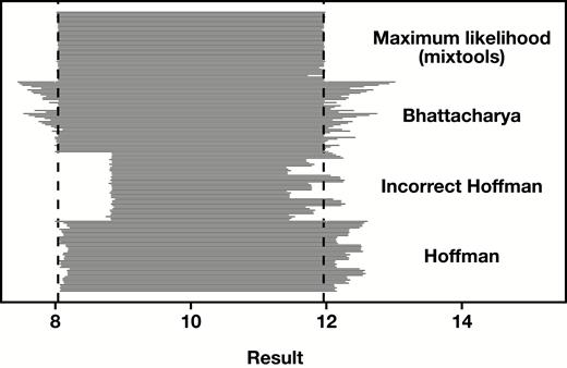
Reference interval estimates across 45 random simulations (n = 100,000 each) as represented by 45 horizontal lines per method spanning the range of the calculated upper and lower limits. The vertical dashed lines represent the target results of 8.04 and 11.96.

In general, our algebraic results and simulations (Figure 5) demonstrate that use of the incorrect variant of Hoffmann’s method will generate reference interval estimates that are too narrow, particularly when $p_H$ is close to 1, the very context in which indirect reference interval strategies are recommended to be constrained.^40,41 This observation has obvious implications for a number of published studies^{8,12-17,19,22} and a reference textbook.¹¹ In addition, there are undoubtedly many unpublished internal studies conducted in clinical laboratories where use of an incorrect method has yielded invalid reference interval estimates.

Some authors, without identifying the use of an incorrect variant, have found fault with the resulting reference intervals and have noted their poor performance in comparison to directly determined values.⁴² Other authors have identified the “linear CDF” variant as a deviation from Hoffmann’s original method^27,43,44 without explicitly specifying the significance. These results have obvious implications for strategies purported to improve the Hoffmann method^14,15 that have used the incorrect variant as a starting point; the proposed refinements have the practical effect of making the flawed variant produce wider reference interval estimates, as Hoffmann’s method would have done.

It must be acknowledged, though, that even when correctly performed, the Hoffmann and other indirect a posteriori methods are imperfect. The International Federation of Clinical Chemistry and Laboratory Medicine Committee on Reference Intervals and Decision Limits has rightly criticized these methods on the basis of their assumption of normality⁴¹ and the errors that inevitably ensue. Likewise, the Clinical Laboratory Standards Institute advises that indirect methods are, at best, tools for rough estimation.⁴⁰

Even when the Gaussian assumption is met, the random simulations we present show that the graphical methods of Hoffmann and Bhattacharya did not perform as well as ML estimates. ML estimates, while sophisticated in their methodology, have been implemented in R and other languages in a manner that is reasonably easy to use. These packages are also capable of simultaneous fitting of multiple modes and in the case of mixdist,³² there is no need to assume the underlying distributions are normal. This affords the fitting of skewed data without application of a normalizing transformation such as Box Cox⁴⁵ (Supplemental Appendix 2).

However, neither the traditional graphical methods nor ML methods represent a panacea for decomposition of mixture distributions. As with any decomposition method, fitted results may not be meaningful from a physiological standpoint. For example, the fitted diseased mode may paradoxically extend well into the range of the healthy or the reference interval estimate may deviate from those established by traditional means. The establishment of a fit that successfully converges and makes clinical sense may require exclusion of extreme outliers or fixing certain parameters as constant (eg, ${\mu }_D$ and/or ${\sigma }_D$⁠) resulting in a solution that is at least, in part, heuristic. This creates the risk that one may introduce arbitrary constraints until one finds what one expects to find. These kinds of trimming assumptions were required to achieve convergent and clinically meaningful fits for both TSH (TSH > 15 mIU/L were excluded) and calcium (results less than the 1st and greater than the 99th percentile of the raw data were excluded), as discussed in Supplemental Appendix 2.

It should be noted that ML fit of Gaussian mixture models has been proposed for the problem of “data mining” reference intervals previously.⁴⁶ However, it is probable that most laboratorians would find the necessary computations intimidating. This motivated our use and provision of open-source R code, which can be applied to mixtures comprised of normal or skewed distributions (see Supplemental Data). It should also be mentioned that other computational strategies employing ML to fit the healthy mode to a truncated normal distribution have been previously described and implemented using custom R code.⁴⁷

Irrespective of the decomposition method, and even when (1) skewing is appropriately accounted for, (2) mixture model decomposition is successful, and (3) fitted model is good, the reference intervals obtained with these procedures may not match what is found in traditional reference interval studies performed on healthy populations. For example, all the decomposition methods assessed yielded lower limits of normal for outpatient male Hb of approximately 11 to 12 mg/dL (110-120 g/L), that is lower than values obtained from healthy populations, which are typically approximately 13.5 to 17.0 g/dL (135 to 170 g/L).⁴⁸ Likewise, the lower limit of normal for uncorrected plasma calcium was also lower than typically reported at approximately 8.0 mg/dL (2.0 mmol/L), which is right on the cusp of levels at which severe symptomatology may appear.⁴⁹

The validity of indirect reference interval estimation is a matter of debate.^43,50 On the basis of our own observations, we believe the recommendation of the Clinical and Laboratory Standards Institute EP28-A3c⁴⁰ is prudent: indirectly calculated reference intervals derived from routine analyses should be used cautiously. What is certain is that if one is to use Hoffmann’s method, it should be undertaken as originally described using a normal QQ plot because use of a linear CDF generates inaccurate and possibly erratic parameter estimates of the healthy mode. However, because more flexible and accurate contemporary computational methods for mixture decomposition are freely available,^32-36 some of which can be performed free of a Gaussian assumption, it may mean that purely graphical procedures like Hoffmann’s have had their day.

Conclusion

The Hoffmann method is frequently applied in a manner divergent from the original description. For distributions satisfying the assumptions of the Hoffmann method, the error of using a CDF plot in linear space rather than a normal QQ plot (equivalent to a normal probability plot) typically leads to reference intervals that are too narrow. The behavior of this erroneous approach is generally dependent on the specifics of the distributions of diseased and healthy individuals and may produce reference intervals that are too wide in select circumstances. Among the methods evaluated (Hoffmann using a QQ plot, Hoffmann using a CDF, Bhattacharya, and ML), ML most consistently recovered the correct values from random number simulations and, depending on the tool employed, has the added benefit of being able to fit skewed distributions without the use of normalizing transformations.