Strong sexual selection despite spatial constraints on extrapair paternity

Abstract

Extrapair paternity should contribute to sexual selection by increasing the number of potential mates available to each individual. Potential copulation partners are, however, limited by their proximity. Spatial constraints may therefore reduce the impact of extrapair paternity on sexual selection. We tested the effect of spatial constraints on sexual selection by simulating extrapair copulations for 15 species of socially monogamous songbirds with varying rates of extrapair paternity. We compared four metrics of sexual selection between simulated populations without spatial constraints and populations where extrapair copulations were restricted to first- and second-order neighbors. Counter to predictions, sexual selection as measured by the Bateman gradient (the association between the number of copulation partners and offspring produced) increased under spatial constraints. In these conditions, repeated extrapair copulations between the same individuals led to more offspring per copulation partner. In contrast, spatial constraints did somewhat reduce sexual selection—as measured by the opportunity for selection, s’_max, and the selection gradient on male quality—when the association between simulated male quality scores and copulation success (e.g., female preferences or male–male competition) was strong. Sexual selection remained strong overall in those populations even under spatial constraints. Spatial constraints did not substantially reduce sexual selection when the association between male quality and copulation success was moderate or weak. Thus, spatial constraints on extrapair copulations are insufficient to explain the absence of strong selection on male traits in many species.

Sexual selection fascinated the earliest evolutionary biologists (Darwin 1871), and it continues to fascinate researchers today because of the complexity of its actions (Cramer et al. 2017; Kaiser et al. 2017) and its potential to contribute to broad-scale patterns in biodiversity (Greig and Webster 2013; Cramer et al. 2016). Considerable work in sexual selection has focused on extrapair paternity (Forstmeier et al. 2014; Arct et al. 2015; Hsu et al. 2015; Brouwer and Griffith 2019), which offers a potential solution to the apparent paradox of sexually dimorphic traits evolving due to selection on male traits in socially monogamous species. Extrapair paternity can lead to strong sexual selection on male traits in socially monogamous species by increasing variance in male mating success, particularly if the preference for male traits is congruent among females (Webster et al. 1995; Neff and Pitcher 2005) or if the trait confers a competitive advantage against other males. However, many studies find weak or no sexual selection on male traits even when extrapair paternity rates are high (Hsu et al. 2015). One hypothesis to explain this contradiction is that spatial constraints on the pursuit of extrapair copulations may limit the opportunity for sexual selection (Canal et al. 2012; Taff et al. 2013; Schlicht et al. 2015; Kaiser et al. 2017). That is, neighboring males can account for close to 75% of identified extrapair sires in some species (Supplementary Table S1; Johnsen et al. 2001; Cramer et al. 2011). Though biased detection of nearby sires may partly explain this pattern (Koenig et al. 1996; Whitaker and Warkentin 2010), rigorous statistical approaches also show that individuals in nearby territories are more likely to perform extrapair copulations together (Canal et al. 2012; Taff et al. 2013; Schlicht et al. 2015; Kaiser et al. 2017). If each male is limited to copulating with neighboring females, copulation success will be distributed across many males in the population rather than restricted to a small subset of males. This distribution of mating opportunities may limit the opportunity for sexual selection and weaken selection on male traits that increase extrapair copulation success (Canal et al. 2012; Taff et al. 2013; Kaiser et al. 2017).

Evaluating the impact of spatial constraints on sexual selection is critical to understanding the interaction of extrapair paternity and sexual selection in a realistic context. However, experimentally manipulating spatial constraints in the wild is logistically challenging and sometimes impossible. Simulations offer a solution. Here, we drew on empirical data from wild populations of 15 socially monogamous songbird species with rates of extrapair paternity that span most of the observed range in passerines (4–54% extrapair offspring in simulated species, Table 1; range in passerines 0–68.5% extrapair offspring; reviewed in Brouwer and Griffith 2019). We simulated extrapair copulations and calculated four complementary and widely applied metrics of the potential for, or strength of, sexual selection. Lastly, we compared the four metrics of selection between populations where extrapair copulations occurred with and without spatial constraints. Because pilot simulations where all males had equal chances of performing extrapair copulations showed little impact of the spatial constraint, we simulated three different degrees of association between an arbitrary male quality trait and copulation success: 1) no association between the two (relevant, e.g., when female preferences are not congruent across females; Fossøy et al. 2008; Arct et al. 2015); 2) a moderate association; and 3) a strong association (relevant, e.g., when female preferences are congruent and strong or when traits are important in male–male competition for extrapair copulations). Scenarios 2 and 3 are those that can generate substantial directional selection on the male trait.

Table 1

Empirical values for extrapair offspring (EPO) and broods containing at least one EPO (EPB) and estimated values of m and s in the 15 songbird species simulated

Species, citation for EPO, EPB, and clutch sizea	% EPO (% EPB)	m, s (n nests for estimation)
Banded wren (Thryophilus pleurostictus; Cramer et al. 2011)	4.0 (10)	0.36, 0.27 (50)
Pied flycatcher (Ficedula hypoleuca; Lehtonen et al. 2009)	4.9 (13.1)	0.18, 0.29 (144)
Great tit (Parus major; van Oers et al. 2008)	6.7 (25.3)	0.45, 0.18 (88)
Blue tit (Cyanistes caeruleus; Charmantier and Perret 2004)	13.2 (50.6)	0.69, 0.23 (104)
House wren (Troglodytes aedon; Cramer 2013)a	13.5 (37.6)	0.80, 0.20 (182)
House martin (Delichon urbica; Whittingham and Lifjeld 1995)a	13.8 (47.4)	0.84, 0.22 (56)
Winter wren (Troglodytes troglodytes; Brommer et al. 2007)	16.3 (37.9)	0.74, 0.26 (29)
Collared flycatcher (Ficedula albicollis; Rosivall et al. 2009)	20.5 (55.7)	0.97, 0.27 (60)
Bluethroat (Luscinia svecica; Fossøy et al. 2008)a	23.6 (45.2)	0.69, 0.44 (261)
Hooded warbler (Setophaga citrina; Stutchbury et al. 1994; Neuhäuser et al. 2001)	27.1 (35.9)	0.48, 0.68 (117)
Willow warbler (Phylloscopus trochilus; Bjørnstad and Lifjeld 1997)a	33.1 (56.3)	0.93, 0.49 (71)
Yellow warbler (Setophaga petechia; Yezerinac et al. 1995)	33.7 (58.8)	1.05, 0.44 (90)
Black-throated blue warbler (Setophaga caerulescens; Kaiser et al. 2015)a	43.4 (55.6)	1.00, 0.59 (1287)
Tree swallow (Tachycineta bicolor; Laskemoen et al. 2010)	47.9 (82.1)	2.00, 0.40 (67)
Reed bunting (Emberiza schoeniclus; Brommer et al. 2007)	52.4 (71.4)	1.37, 0.61 (70)

Parameters m and s used in simulating these species (see main text) were estimated by Brommer et al. (2010) for flycatchers and tits and using their code for other species based on the distribution of extrapair offspring within nests.

^aUnpublished data associated with publications were used: ERAC (house wrens); Jan Lifjeld (willow warblers, house martins); Arild Johnsen (bluethroats); SAK, Scott Sillett and Mike Webster (black-throated blue warblers); and ERAC, Michelle Hall and Sandra Vehrencamp (banded wrens).

METHODS

We modeled spatially constrained and spatially unconstrained extrapair copulations using three levels of association between male quality and copulation success and treating copulation and fertilization as separate steps in reproduction. For each simulated population, we began with 400 male–female breeding pairs on equally sized territories arranged in a 20 × 20 grid (i.e., study plot), where the unit of measurement was territory diameters. When simulating spatial constraints, we allowed only first- and second-order neighbors to be extrapair copulation partners and weighted copulation probability by distance (see below). We excluded males with territories three units or less from the edge of the grid from the final data sets to avoid edge effects in models with spatial constraints and for consistency in the unconstrained conditions.

We assigned each male a quality score (absolute male quality) drawn from a normal distribution with a mean of 0 and a standard deviation (SD) of 1. These quality scores are intended to reflect “good genes” traits, underlain by additive genetic variation (Neff and Pitcher 2005). Our simulation approach required all values to be positive, and the pilot work (not shown) indicated that strong associations between male quality and copulation success occurred only when skew in male copulation success was substantial. We therefore shifted the male quality distribution to have a minimum of 0.1 and assigned each male a copulation likelihood score by raising his quality score to a power of 0, 3, or 9. This process created three levels of association between male quality and copulation success, which we also refer to as copulation skew (no, moderate, and strong associations, respectively). Note that all males had equal copulation likelihood scores for the models with no copulation skew.

To simulate extrapair copulations, we drew a value E, representing the number of extrapair copulations performed by each female, from a Poisson distribution with the species-specific mean m (see below; Brommer et al. 2007, 2010; values of m for the 15 simulated species listed in Table 1). For the model with copulation skew 0, E was random with respect to the quality of the within-pair male. For copulation skew 3 and 9, females paired to high-quality males performed fewer extrapair copulations. We sorted a list of 400 values of E in increasing order, sorted males in decreasing order of quality, and assigned E to females based on the within-pair male’s position on the list. Absolute male quality was used for spatially unconstrained models, and relative quality (the difference between the within-pair male and the mean of his first- and second-order neighbors) was used in spatially constrained models, as the social context of the male may alter copulation success (McDonald et al. 2013; Cramer et al. 2017).

Each female then drew, with replacement, the identity of the E extrapair copulation partners. Candidate partners were the entire population (unconstrained models) or males with territories less than 2.5 territory units away (i.e., immediate and second-order neighbors only; constrained models). We used the sample function of program R v. 3.3.0 (R Development Core Team 2012), whereby a male’s probability of being drawn as a copulation partner was proportional to his weighting value relative to the sum of the values of all other candidate extrapair copulation partners. Weighting values were equal to the male’s copulation likelihood score (unconstrained models) or to the product of his copulation likelihood score and the inverse of the squared distance between the male’s territory and the location of the focal female (constrained models).

After simulating copulations, we simulated fertilizations. Female clutch size was drawn with replacement from the empirical distribution of clutch sizes for each species (data sources in Table 1). Each egg in a female’s clutch was assigned as being sired by the within-pair or extrapair male by drawing from a Bernoulli distribution with a mean f, calculated separately for each female by the following equation:

$${\displaystyle \begin{array}{l}{\displaystyle f=\frac{E\times s}{E\times s+(1-s)}}\end{array}}$$

(1)

where s is a species-specific parameter that describes the number of sperm contributed by a single extrapair copulation relative to the total number of sperm inseminated by the within-pair male (which is assumed to be constant across males; values estimated by Cramer et al. in review; Brommer et al. 2010; Table 1; equation 3 of Brommer et al. 2007). For each egg fertilized by an extrapair male, we drew the identity of the sire with replacement from the female’s extrapair copulation partners. This procedure approaches a fair raffle among the extrapair males (Parker 1990), with sperm from any extrapair copulation having an equal likelihood of fertilizing the egg.

Estimating parameters

The model parameters we use, m and s, were introduced by Brommer et al. (2007, 2010), in order to generate a realistic null distribution of extrapair offspring among nests. The two parameters can be simultaneously estimated using data on the number of extrapair offspring in nests of different clutch sizes. For a value of m, the distribution of values of E is known from the Poisson distribution. For each value of E and each clutch size, the expected number of extrapair offspring can be calculated using the probability mass function of the binomial distribution, with the mean of the binomial determined by s and E following Equation 1. Using a Bayesian process, m and s are simultaneously optimized to produce the best fit to the empirical distribution of extrapair offspring among nests. This process assumes that each extrapair copulation is independent, and it produces realistic distributions for most species tested (Supplementary Table S2; Cramer et al. in review; Brommer et al. 2007, 2010). We used values of m and s from Brommer et al. (2010) for the four species in that paper, choosing one population that appeared representative of the species. For the remaining 11 species, we obtained data on the distribution of extrapair offspring within clutches (species and sources in Table 1) and estimated m and s (see also Cramer et al. in review). To do so, we used code from Brommer et al. (2010) in JAGS (Plummer 2003), accessed through Program R v. 3.3.0 (R Development Core Team 2012) using rjags (Plummer et al. 2016) and jagsUI (Kellner 2016). Empirically evaluating the accuracy of m and s is not feasible under typical field study conditions. However, our results with respect to the impact of spatial constraints on selection were unchanged in pilot simulations where values of m and s were allowed to randomly and independently vary up to 10% above or below their estimated values (results not shown but replicable using our code archived in Dryad).

Analyzing populations

After we assigned paternity to all offspring in the population, we calculated the total number of genetic offspring for all males (i.e., total reproductive success). Extrapair offspring sired in territories close to the edge of the study plot were included in total reproductive success for focal males, although males in these edge territories were removed from further analyses for both constrained and unconstrained models. We calculated four selection metrics for each population. 1) Opportunity for selection reflects the maximum possible strength of selection in the population and was calculated as the population-wide variance in reproductive success divided by the squared mean of reproductive success (Crow 1958; Arnold and Wade 1984). This metric, and derivatives of it, have been widely applied in extrapair paternity studies (e.g., Freeman-Gallant et al. 2005; Webster et al. 2007). 2) The Bateman gradient reflects the strength of selection to copulate with multiple individuals (Bateman 1948) and was measured as the slope parameter from regressing the number of offspring on the number of copulation partners. The within-pair mate was included as a copulation partner regardless of whether they produced offspring together. 3) s’_max is the maximum possible sexual selection differential on a trait and was calculated as the product of the relativized Bateman gradient with the square root of standardized variance in the number of copulation partners (Jones 2009). The Bateman gradient was relativized by dividing total reproductive success and the number of copulation partners by their population means before performing the regression. Standardized variance in the number of copulation partners was the variance in this value, divided by its mean squared (Jones 2009). While s’_max has not been widely applied as of yet, it best reflects the intuitive strength of sexual selection in simulated populations with different social mating systems (Henshaw et al. 2016). 4) The selection gradient on male quality estimates the strength of selection acting on a trait (Lande and Arnold 1983). It was calculated as the coefficient from regressing the standardized number of offspring on the standardized male quality score (Lande and Arnold 1983). Male quality was standardized to have a mean of 0 and an SD of 1. The number of offspring was standardized by dividing by the population mean (Lande and Arnold 1983). Of these metrics, the selection gradient most directly measures the strength of selection on male traits, the focus of this study, but it can only be assessed when the target of selection is known. A benefit of the other three “proxy” metrics is that they can be assessed for a study population even if the target of selection is not known (Henshaw et al. 2016). Note that we had complete information on copulation partners in our simulations; a typical field study might instead infer copulation partners based on the genetic parentage of offspring, which can result in biased estimates, particularly for the Bateman gradient and s’_max (Cramer et al. in review).

Statistical analyses

In total, we simulated 600 populations of each of the 15 species (Table 1): 100 replicate populations for each of the six conditions (copulation skew 0, 3, and 9, with and without spatial constraints). We tested whether metric values differed depending on spatial constraints by constructing a separate linear mixed model for each metric and each level of copulation skew. Species was a random effect and spatial constraint was the fixed effect. To assess the effect size of spatial constraints, we calculated Cohen’s d, following equation 22 in Nakagawa and Cuthill (2007) to account for nonindependence within species. Following their recommendation, effect sizes less than 0.2 are interpreted as small. Correction for multiple testing using either false discovery rate or Bonferroni correction did not affect significance decisions (raw P-values are shown). To confirm that increasing the copulation skew increased measured selection, we ran linear mixed models using the spatially constrained data only, with copulation skew as a categorical fixed effect and species as a random effect. It was not possible to combine this analysis with the analysis of the spatial effect due to problems with model convergence. Furthermore, we compared whether selection was stronger with spatial constraints and a high copulation skew (value of 9) or with no spatial constraints and a moderate copulation skew (value of 3) by running a model with the data set restricted to contain only these two subsets of simulated populations. Models were run with lme4 (Bates et al. 2015), with significance assessed in lmerTest (Kuznetsova et al. 2017). Average values for each species were visualized using ggplot2 (Wickham 2016) in program R v. 3.3.0 (R Development Core Team 2012). Except where noted, analysis of mean values instead of individual replicate populations produced similar results for linear mixed-model results.

To test whether selection metrics were higher in species with higher extrapair paternity, we assessed the correlation between mean metric values and empirical values of the percentage of extrapair offspring in each species. To minimize multiple testing, we a priori chose to use data only from simulations with copulation skew 9 and unconstrained copulations, where the between-species variance in metric values appeared greatest. We also assessed whether spatial constraints had a stronger impact on sexual selection metrics in species with more extrapair paternity by testing whether the empirical percentage of extrapair offspring for each species correlated with the difference in mean sexual selection metrics between spatially constrained and unconstrained conditions (copulation skew 9 only).

RESULTS

Three of the sexual selection metrics—opportunity for selection, s’_max, and the selection gradient—did not differ significantly between spatially constrained and unconstrained conditions with copulation skew 0 (no association between male quality and copulation success; Table 2). In models with copulation skew 3 and 9 (moderate and strong associations between male quality and copulation success; Table 2), all four metrics, including Bateman gradient, differed significantly between spatially constrained and unconstrained models. Opportunity for selection, s’_max, and the selection gradient were higher in unconstrained models, and the Bateman gradient was higher in constrained models (Table 2; Figure 1). However, for all four metrics, effect sizes were low (Cohen’s d < 0.2) for models with copulation skew 0 and 3 (Table 2).

Table 2

Comparison of spatially constrained (C) and unconstrained (U) models with different strengths of association between male quality and copulation success (copulation skew) for four sexual selection metrics

Selection metric	Copulation skew	F-test results	Metric (mean ± SE) in C model	Difference (mean ± SE) in metric in U model	Effect size of spatial constraint (Cohen’s d)
Opportunity for selection	0	F1,2984 = 2.40, P = 0.12	0.25 ± 0.03	0.00 ± 0.00	0.02
	3	F1,2984 = 20.81, P < 0.001	0.39 ± 0.06	0.01 ± 0.00	0.04
	9	F1,2984 = 126.07, P < 0.001	0.95 ± 0.25	0.40 ± 0.04	0.29
Bateman gradient	0	F1,2984 = 20.59, P < 0.001	0.55 ± 0.06	−0.01 ± 0.00	−0.05
	3	F1,2984 = 103.30, P < 0.001	0.72 ± 0.08	−0.03 ± 0.00	−0.08
	9	F1,2984 = 1154.47, P < 0.001	0.70 ± 0.07	−0.10 ± 0.00	−0.32
s’max	0	F1,2984 = 1.22, P = 0.27	0.26 ± 0.03	0.00 ± 0.00	0.01
	3	F1,2984 = 18.34, P < 0.001	0.43 ± 0.06	0.01 ± 0.00	0.04
	9	F1,2984 = 109.18, P < 0.001	0.79 ± 0.12	0.11 ± 0.01	0.20
Selection gradient	0	F1,2998 = 0.16, P = 0.69	0.00 ± 0.00	0.00 ± 0.00	0.01
	3	F1,2984 = 70.06, P < 0.001	0.37 ± 0.05	0.01 ± 0.00	0.08
	9	F1,2984 = 493.83, P < 0.001	0.53 ± 0.08	0.09 ± 0.00	0.29

Figure 1

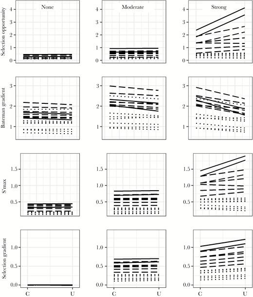
Opportunity for selection (top row), Bateman gradient (second row), s’_max (third row), and selection gradient (bottom row) on male quality in 15 simulated species of songbirds with and without spatial constraints on extrapair copulation behavior. Simulations were run in which male quality was not associated with copulation success (left column; copulation skew 0), was moderately associated (middle column; copulation skew 3), or was strongly associated (right column; copulation skew 9). Each line connects mean values across 100 simulated populations of a single species in spatially constrained (C) and unconstrained (U) mating conditions. Species for which less than 20% of offspring are sired by extrapair males are in dotted lines; 20–40% offspring sired by extrapair males are in dashed lines; and 40–60% offspring sired by extrapair males are in solid lines (categorized using empirical values).

Sexual selection metrics generally increased with increasing copulation skew (F_2,4483 > 1970, P < 0.001; comparisons of consecutive values, |t₄₄₈₃| > 12.6, P < 0.001), except for the Bateman gradient, which did not differ between copulation skew 3 and 9 (t₄₄₈₃ = 0.94, P = 0.35). In models using the average value per simulation condition set, the difference in opportunity for selection was not significant between copulation skew 0 and 3. Notably, the impact of copulation skew on sexual selection metrics was greater than the impact of spatial constraints: selection was stronger in the constrained models with copulation skew 9 than in the unconstrained models with copulation skew 3 (opportunity for selection F_1,2984 = 2186.4, t₂₉₈₄ = 46.76, P < 0.001; s’_maxF_1,2984 = 4608.7, t₂₉₈₄ = 67.89, P < 0.001; selection gradient F_1,2984 = 1914.5, t₂₉₈₄ = 43.76, P < 0.001; not tested for Bateman gradient).

Sexual selection metrics were higher in species with higher percentage of extrapair offspring (using mean metric values from spatially unconstrained simulations with copulation skew 9: opportunity for selection: t₁₃ = 14.56, P < 0.001, Pearson r = 0.97; Bateman gradient: t₁₃ = 2.22, P = 0.04, r = 0.52; s’_max: t₁₃ = 29.09, P < 0.001, r = 0.99; selection gradient: t₁₃ = 21.82, P < 0.001, r = 0.99; see line types in Figure 1). The effect of the spatial constraint (i.e., the difference in sexual selection metrics across spatial conditions) was higher for species with higher percentage of extrapair offspring (Figure 2; copulation skew 9 only; opportunity for selection: t₁₃ = 7.48, P < 0.001, Pearson r = 0.90; Bateman gradient: t₁₃ = −6.40, P < 0.001, r = −0.87; s’_max: t₁₃ = 7.69, P < 0.001, r = 0.91; selection gradient: t₁₃ = 13.41, P < 0.001, r = 0.97).

Figure 2

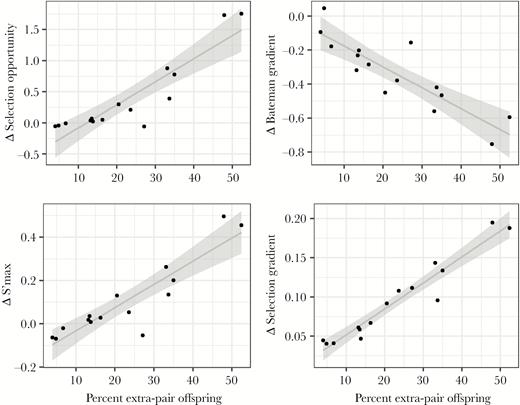
Differences in sexual selection metrics between spatially constrained and unconstrained conditions as a function of empirical percent extrapair offspring across 15 simulated species with a strong association between male quality and copulation success. The line shows the estimated regression, while shading indicates the 95% confidence interval.

Detailed descriptions of the distribution of sexual selection metrics, extrapair copulations, and extrapair offspring for each simulated condition and species are given in Supplementary Table S2. For opportunity for selection, s’_max, and the selection gradient, among-replicate variation appeared to increase in models with higher copulation skew (see SD and 95% confidence intervals in Supplementary Table S2). Among-replicate variation in the Bateman gradient, in contrast, was relatively similar across models with different copulation skew (Supplementary Table S2).

DISCUSSION

Our simulations show that strong sexual selection can occur despite substantial spatial constraints on extrapair copulations. Spatial constraints somewhat reduced sexual selection in models where the association between male quality and copulation success (here called copulation skew) was strong, although selection on male traits (measured as the selection gradient) remained strong in these models. Spatial constraints had a negligible impact on sexual selection in models where copulation skew was moderate (which generated substantial selection gradients on male traits) or nonexistent, and in species with low rates of extrapair paternity.

High-quality males performed the majority of extrapair copulations when these copulations were spatially unconstrained and there was high copulation skew. In contrast, a high-quality male could dominate copulations only within a limited subset of the female population (i.e., nearest neighbors) when copulations were spatially constrained. Thus, the variance in male reproductive success (i.e., opportunity for selection) was reduced under spatial constraints, as was s’_max and the strength of selection on the male quality trait, as previous studies hypothesized (Canal et al. 2012; Taff et al. 2013; Schlicht et al. 2015; Kaiser et al. 2017). However, spatial constraints did not substantially affect these three selection metrics in models with moderate or no copulation skew (i.e., moderate or no association between male quality and copulation success). In these models, without spatial constraints, each male had a low likelihood of copulating with any one female, but many females were potential copulation partners. With spatial constraints, males had a higher likelihood of copulating with neighboring females, but the number of potential copulation partners was reduced. Due to the probabilistic way we assigned copulations, the elevated likelihood of copulation for higher-quality males in the moderate model was not sufficient for these males to dominate copulations in either spatially constrained or unconstrained conditions. As a result, spatial constraints had little impact on the opportunity for selection, s’_max, or the selection gradient in the models with moderate copulation skew, even though the realized strength of selection on male quality traits (the selection gradient) was still quite high.

In contrast to how spatial constraints prevented individual males from dominating copulations across populations of females, spatial constraints allowed high-quality males to dominate extrapair copulations within individual females. That is, under spatial constraints, males were more likely to obtain multiple copulations with the same extrapair female, which increased the number of extrapair offspring they sired per female, increasing the Bateman gradient compared to spatially unconstrained conditions (Supplementary Table S2). Repeated copulations with the same extrapair partner were most likely in models where the copulation skew was high and copulations were spatially constrained. Repeated copulations became less likely either when copulations were unconstrained spatially (increasing the number of potential copulation partners) or when the association between male quality and copulations success weakened (i.e., copulation skew decreased, decreasing the degree to which individual males dominated available copulations). Our models assumed that each extrapair copulation was independent of whether those individuals had previously copulated. If individuals preferentially remate, or preferentially avoid remating, with the same extrapair copulation partners, the effect of spatial constraints on the Bateman gradient in real populations may differ. Direct evidence on repeated copulations between extrapair partners is limited, but extrapair sires often differ between consecutive broods by the same female within a breeding season (Stutchbury et al. 1994; Bouwman et al. 2006). The degree to which each extrapair copulation depends on previous copulations deserves more study. Regardless, our results highlight a difficulty in interpreting the Bateman gradient, as the number of offspring produced may be better predicted by the number of copulations a male performs rather than the number of copulation partners (the variable used in the Bateman gradient).

In addition, the Bateman gradient did not reflect the intuitive strength of sexual selection, as found in a previous study (Henshaw et al. 2016). Specifically, the Bateman gradient did not increase across models with increasing copulation skew. Moreover, the Bateman gradient was not highly correlated with the percentage of extrapair offspring in the species, although the percent of extrapair offspring was highly correlated with the selection gradient, a direct measure of selection (note that line types representing different rates of extrapair offspring do not sort neatly for the Bateman gradient in Figure 1). The relative weakness of the correlation is likely because of the complexity of factors affecting the Bateman gradient. This metric depends on the balance between the number of within-pair offspring and the number of extrapair offspring per copulation and how these values are distributed across males. Both within-pair and extrapair offspring depend, in turn, on clutch size and the relative impact of sperm competition, with within-pair offspring also depending on the number of extrapair copulations a male’s social mate performed. Thus, we contribute to a growing body of literature raising issues with the Bateman gradient: that it is not intuitively related to sexual selection (Henshaw et al. 2016); that it does not adequately separate precopulatory and postcopulatory, prezygotic selection (Tang-Martinez and Ryder 2005); that it does not separate correlation and causation (Anthes et al. 2016); and that it can be strongly biased due to sampling limitations in typical field studies (Cramer et al. submitted).

Unlike the Bateman gradient, opportunity for selection, s’_max, and the selection gradient were higher in models where copulation skew (i.e., the association between male quality and copulation success) was highest. As expected, no sexual selection, as measured by these three metrics, was detected in models where copulation skew was 0. Selection gradients in our models were fairly strong relative to average reported empirical values for traits related to mating and fecundity (where empirically observed average values typically are less than 0.3; Kingsolver et al. 2012). Stronger sexual selection in our simulations may result from complete success in all nesting attempts (i.e., no loss of offspring through depredation and/or weather events, which add noise to empirical data sets relating male quality to reproductive success), as well as from our methods for associating male quality with both cuckoldry and extrapair copulation success. It is difficult to assess how realistically our simulations recreated processes that occur in the wild, as insufficient data are available on the mechanisms linking male sexual traits to copulation success. Broad-scale questions remain open in many species on whether associations between male sexual traits and copulations are driven by female choice or by male–male competition (Forstmeier et al. 2014) and to what degree variation in male quality correlates with extrapair mating success (Hsu et al. 2015). Generally, many males in a population sire extrapair offspring, suggesting some level of stochasticity or noncongruence in female choice, which our simulation procedure captures (Supplementary Table S2). The most realistic models for associating male quality and copulation success, however, likely vary among species, populations, and years (e.g., Chaine and Lyon 2008). Rather than argue that any one of our models is best for a given species, we suggest that sexual selection on male traits will be less impacted by spatial constraints in species with weaker or less congruent female choice or male–male competition.

The spatial constraint we model here is relatively strong, as all extrapair sires were first- or second-order neighbors. For comparison, studies on banded wrens (Cramer et al. 2011) and bluethroats (Johnsen et al. 2001) found that approximately 75% of assigned extrapair sires were within this radius, and some extrapair sires could not be identified (as is true for many studies). Identified sires may be more likely to be close territorial neighbors than are unidentified sires, for example, if unassigned fathers are males with territories outside the study site (Whitaker and Warkentin 2010). Thus, the simulated spatial constraint is likely to be more restrictive than is typically observed in nature. Because our simulated spatial constraint is likely stronger than that experienced by most species, and because pilot models with even stronger spatial constraints gave similar results (data not shown but replicable using our code archived in Dryad), it is unlikely that spatial constraints on extrapair copulations would have a stronger impact on sexual selection metrics than what we observed here.

Previous work suggesting that spatial constraints on extrapair copulations limit sexual selection have considered male traits that are expected to be under directional selection, where males with high trait values are more likely to obtain copulations with females regardless of female identity. Our simulations included populations with no association between the male quality trait and copulation success for completeness, and because female preferences may sometimes be noncongruent, for example, in species where extrapair copulations depend on the genetic similarity of the male and the female (Fossøy et al. 2008; Arct et al. 2015). In such species, directional selection on a male quality trait is not expected, as a typical male quality trait cannot capture similarity to all females in the population. Rather, we might expect balancing or diversifying selection on male genotypes. Whether spatial constraints influence the strength of such nonlinear selective forces on male genotypes was beyond the scope of this paper. The lack of an effect of spatial constraint on directional selection on the male quality trait in these models, although not an a priori expectation, is perhaps unsurprising.

Spatial constraints have further been hypothesized to impact the extent to which extrapair paternity occurs. For example, limitations on extraterritorial forays may explain the dramatic evolutionary loss of extrapair copulation in the purple-crowned fairy-wren (Malurus coronatus), which lives under particularly strong spatial constraints (Kingma et al. 2009). Adequately simulating the impact of spatial constraints on the frequency of extrapair paternity would require extensions to the current model, for example, assigning variation in offspring fitness as a function of the quality of their sires and assigning distance-based costs to off-territory foray behavior. This was beyond the scope of the current analysis, but our models lay the groundwork for further exploration by giving us a better understanding of the interaction between sexual selection and spatial constraints given constant extrapair copulation rates.

CONCLUSIONS

As hypothesized (Canal et al. 2012; Taff et al. 2013; Kaiser et al. 2017), spatial constraints reduce sexual selection on male traits, but the magnitude of the reduction is small relative to the magnitude of selection. Thus, it is unlikely that spatial constraints moderate the strength of sexual selection severely and consistently enough to explain the absence of consistent associations between male quality traits and extrapair paternity in many species (Akçay and Roughgarden 2007; Hsu et al. 2015). This finding revitalizes the mystery of what guides extrapair paternity success in many species where the association between male traits and mating success is unclear.

FUNDING

There is no funding to report.

Acknowledgments

We thank Arild Johnsen, Jan Lifjeld, Scott Sillett, Mike Webster, Michelle Hall, and Sandra Vehrencamp for sharing unpublished data on clutch size and distribution of extrapair offspring among nests. Emmi Schlicht and an anonymous reviewer provided comments that improved the quality of the paper.

Data accessibility: Analyses reported in this article can be reproduced using the data provided by Cramer et al. (2020).