A multilevel society of herring-eating killer whales indicates adaptation to prey characteristics

Abstract

Non-social factors can influence animal social structure. In killer whales (Orcinus orca), fish- versus mammal-eating ecological differences are regarded as key ecological drivers of their multilevel society, including group size, but the potential importance of specific target prey remains unclear. Here, we investigate the social structure of herring-eating killer whales in Iceland and compare it to the described social structures of primarily salmon- and seal-eating populations in the Northeast Pacific, which form stable coherent basic units nested within a hierarchical multilevel society. Using 29023 photographs collected over 6 years, we examined the association patterns of 198 individuals combining clustering, social network structure, and temporal patterns of association analysis. The Icelandic population had largely weak but non-random associations, which were not completely assorted by known ranging patterns. A fission–fusion dynamic of constant and temporary associations was observed but this was not due to permanent units joining. The population-level society was significantly structured but not in a clear hierarchical tier system. Social clusters were highly diverse in complexity and there were indications of subsclusters. There was no indication of dispersal nor strong sex differences in associations. These results indicate that the Icelandic herring-eating killer whale population has a multilevel social structure without clear hierarchical tiers or nested coherent social units, different from other populations of killer whales. We suggest that local ecological context, such as the characteristics of the specific target prey (e.g., predictability, biomass, and density) and subsequent foraging strategies may strongly influence killer whale social association patterns.

INTRODUCTION

The sociality of a group-living species is driven by a trade-off between its specific ecological, evolutionary, and social contexts (Krause and Ruxton 2002). Non-social factors, particularly predation risk, finding/catching food, defending resources, and resource patchiness, can strongly determine the social structure of simple social systems and provide the context for the development of complex ones (Jarman 1974; Wrangham 1980; Whitehead 2008a). General socioecological frameworks have been developed for various taxa, characterizing how such factors can affect sociality by using broad characteristics of a species/genera, such as occurrence of group foraging, group size or mating system (Emlen and Oring 1977; Wrangham 1980; Gowans et al. 2007). However, with the increase of within-species studies (e.g., Barton et al. 1996, Sinha et al. 2005; Whitehead et al. 2012), it seems clear that it is important to emphasize intraspecific variation which likely reflects variability under different ecological conditions. Investigating different populations of the same species across ecological gradients is therefore valuable to evaluate the influence of ecological drivers.

Multilevel societies are among the social systems found on group-living species and have been described as hierarchical structures of nested social levels (i.e., discrete social stratification of associations among individuals into tiers) with at least 1 stable core unit (Wittemyer et al. 2005; Grueter et al. 2012a; Grueter et al. 2012b). Recently, de Silva and Wittemyer (2012) suggested that multilevel societies should be seen along a continuum of nestedness and that some might present less clearly hierarchically stratified social levels that transition more gradually. Commonly, multilevel societies exhibit fission–fusion dynamics, with frequent association, disassociation, and reassociation of groups of individuals (e.g., Connor et al. 1992). Although multilevel societies have been studied more extensively in terrestrial mammals, particularly in primates (see Grueter et al. 2012a), such social systems are also observed in cetaceans and intraspecific variation has been reported (Connor et al. 1998; Whitehead et al. 2012). For example, female sperm whales (Physeter macrocephalus) form long-term stable social units which, in the Pacific, temporarily group with other units with which they share part of the acoustic repertoire, but rarely group in the North Atlantic, possibly due to differences in predation risk (Whitehead et al. 2012).

One well-described tiered multilevel society among cetaceans is that of the “resident” fish-eating killer whale (Orcinus orca) population in the Northeast Pacific, hereafter termed residents. The basic unit of this society is the matriline, consisting of an oldest surviving female and her philopatric descendants, remaining associated with their mother for life (Bigg et al. 1990; Baird and Whitehead 2000; Barrett-Lennard 2000). Within matrilineal units, individuals associate strongly and at very similar levels, whereas matrilineal units can frequently interact (Bigg et al. 1990; Baird and Whitehead 2000; Ford et al. 2000). Matrilines that share at least part of their acoustic repertoire, probably due to common maternal ancestry, form the next social level, the clan (Ford 1991). Different clans have no calls in common, and matrilines from the same or different clans frequently travel together (Ford 1991). The next and broadest social level (just under population) is the community, consisting of matrilines that share a common area and associate periodically but not with those of another community (Bigg et al. 1990). This multilevel society is based on distinct fission–fusion patterns of whole coherent family based units, where stable matrilineal units collectively associate more frequently with other close kin units. The “sub-pod” and “pod” were traditionally considered intermediate social levels between the matriline and the clan, consisting of matrilines with recent maternal ancestry that often (>95% and 50% of the time, respectively) travelled together (Bigg et al. 1990; Ford 1991). However, recent studies have shown fluctuations in the reoccurrence of associations between matrilines (Ford and Ellis 2002; Parsons et al. 2009), as well as changes in the pods originally described (Ford et al. 2000), leading to suggestions that the term “pod” should only be used to designate aggregations of killer whales or as a synonym for matriline (Ford and Ellis 2002).

Intraspecific variation in sociality among killer whales is believed to relate to prey-type. Northeast Pacific resident killer whales mainly prey on salmon, especially Chinook (Oncorhynchus tshawytscha) while mammal-eating killer whales (also referred to as “transients” or Bigg’s killer whales) feed on marine mammals, especially harbour seals (Phoca vitulina; Ford et al. 1998). Although sympatric, these 2 populations comprise 2 specialist ecotypes that are socially and reproductively segregated (Bigg 1982; Barrett-Lennard 2000). Both ecotypes exhibit coherent and stable matrilineal social units based on long-term kinship associations but there are important distinctions between their social strategies. The resident population forms larger matrilineal units than the mammal-eating population and while the resident population is philopatric, there is some level of adult dispersal in the mammal-eating population (Bigg et al. 1990; Baird and Whitehead 2000). For example, males may disperse to briefly associate with other matrilines or live alone, randomly associating with other adult males. Moreover, some females may disperse from the matriline and stay socially mobile, associating strongly for short periods with different groups (Baird and Dill 1996; Baird and Whitehead 2000). This variation is considered to be due to the different foraging strategies of the populations. Hunting marine mammal prey in large groups incurs greater costs by increasing the probability of detection by the prey. Furthermore, the optimal energetic intake for mammal-eating killer whales (preying upon medium-sized seals) declines for groups larger than 3 individuals (Baird and Dill 1996). In contrast, resident killer whales spread out and coordinate to locate salmon (Ford et al. 2000), potentially benefiting from larger group sizes. With little or no predation risk, populations of this species apparently refine their social systems primarily in relation to foraging efficiency, particularly availability of resources and competition for those resources.

In the North Atlantic, the only published study addressing sociality found greater similarities between the Scottish mammal-eating population and Northeast Pacific mammal-eating population relative to residents, despite greater phylogenetic distance, suggesting that ecology drives sociality more than phylogenetic inertia does (Beck et al. 2012). The study included a limited dataset from Icelandic herring-eating killer whales and their social structure was not explored in detail. However, the study’s hierarchical display of associations suggested that social tiers were not clearly defined in this population and that associations at a variety of strengths existed. These features were not further addressed, nevertheless the study concluded that the Icelandic fish-eating population is probably more similar to the Northeast Pacific resident population than to mammal-eating populations.

Icelandic killer whales are believed to mainly prey upon Atlantic herring (Clupea harengus) and follow the Icelandic summer-spawning (ISS) herring stock during its yearly migration (Sigurjónsson et al. 1988) between overwintering, feeding and spawning grounds (Óskarsson et al. 2009). Unlike the salmon prey of resident killer whales, herring form large and dense schools as an antipredator strategy (Nøttestad and Axelsen 1999) and killer whales feeding on herring schools use a coordinated group feeding strategy, encircling their prey to herd and capture it (Similä and Ugarte 1993). Feeding aggregations of killer whales are very common in Iceland, making it difficult to discern isolated groups and confusing the determination of associations in the field (Sigurjónsson et al. 1988; Beck et al. 2012). In addition, herring can undergo large variations in abundance and migration routes (Jakobsson and Stefánsson 1999; Óskarsson et al. 2009) making it a changeable food resource. In fact, recent research suggests not all individuals specialize on ISS herring and follow it year-round. Other killer whales observed only in 1 season or seasonally moving between Iceland and Scotland exhibited wider trophic niche width, suggesting diversity in foraging strategies (Samarra and Foote 2015; Samarra et al., 2017; FIP Samarra et al. in prep).

In this study we investigate the social structure of herring-eating killer whales in Iceland, based upon patterns of association among photo-identified individuals in spawning and overwintering grounds. We relate our results to the described societies of killer whales in the Northeast Pacific. Specifically, we investigate: 1) the degree and diversity of associations between pairs of individuals; 2) whether social structural units of individuals exist and are hierarchically nested in the social structure; 3) how associations persist or change over time in the population and depending on age–sex class; and 4) whether variations in movement and feeding strategy within the Icelandic killer whale population influence sociality by promoting social segregation. Given the differences in historical availability, migration patterns, and antipredator strategies of herring, salmon, and seals, we hypothesize that broad ecology (fish- vs. mammal-eating) alone cannot explain sociality and that local ecological conditions, such as characteristics of prey schools and associated foraging strategy of the population, might also strongly shape the social structure of killer whales.

METHODS

Data collection

Photographs of killer whales were collected in July 2008–2010 and 2013–2015 in Vestmannaeyjar (South Iceland), a spawning ground of ISS herring, and in February–March 2013–2014 and mid-February to mid-March 2015 in Grundarfjörður and Kolgrafafjörður (West Iceland), 2 fjords that were part of the ISS herring overwintering grounds. During daylight hours, when killer whales were encountered, groups were approached and photographs of all individuals surfacing together were taken using a variety of digital single-lens reflex cameras with telephoto lenses. On several occasions, more than 1 photographer/camera was used. Sampling effort varied across years and seasons, due to weather conditions, research effort priorities, and the number of research vessels used (Table 1). In the winters of 2014–2015, a whale-watching platform was also used. Due to the inherent difficulty in approaching and photographing all individuals from whale watching platforms, only encounters when coverage of the groups present was considered complete (i.e., all individuals in the group were identified) were included in the analysis.

Table 1

Summary of the photo-identification sampling effort included in this study

Year	Season	Sampling periods used (days)		Start–end of sampling periods	Number of
		Research vessels	WW platform		Photographs	Identified individuals
2008	Summer	6	—	8th–20th July	382	29
2009	Summer	16	—	7th–29th July	2552	65
2010	Summer	6	—	4th–10th July	748	70
2013	Winter	23	—	10th February–24th March	5649	211
	Summer	4	—	17th–29th July	1980	51
2014	Winter	19	1	13th February–31st March	5510	115
	Summer	15	—	6th–27th July	5265	149
2015	Winter	—	1	1st March	118	3
	Summer	19	—	7th–29th July	6819	131

Days of sampling are discriminated by type of platform: research vessels and whale-watching (WW) boat.

Photo-identification

Killer whales were individually identified based on the size and shape of the dorsal fin, patterns of the saddle patch, and natural markings, such as nicks and scars, using left-side pictures (Bigg 1982). For young animals without distinct natural markings, the eyepatch was also used for identification across seasons/years. The quality of photographs was judged based upon focus, contrast, angle and overall quality assessment (adapted from Friday et al. 2000). Only high and medium quality photographs were used. To avoid false positives, matches were confirmed if 3 distinct features of the individual were unambiguously identified.

To differentiate sex and stage of maturity 4 different categories were used: 1) adult males—adults that have reached sexual maturity and present distinguishably taller dorsal fin; 2) adult females—mature size individuals, with relatively smaller dorsal fin, seen during the study period either consistently with a calf in echelon position, or without developing dorsal fin for at least 3 years, or that were matched to a preliminary catalogue from the Marine Research Institute including photos taken between 1981 and 2007, without developing dorsal fin; 3) juveniles—identifiable individuals >1 year old that have not reached mature size (both sexes); 4) other—whales of apparently larger size than juveniles but for which sex and stage of maturity were impossible to determine.

Individuals that were only sighted in the summers of 2008–2010 were excluded from the analysis to reduce bias resulting from including individuals that may have died during the first years of the study and reduce the possibility of incomplete group coverage data from fieldwork where photographic data collection was opportunistic. This procedure excluded 25 individuals from the study.

Association criterion

Due to the common observations of aggregations of individuals in Iceland (Sigurjónsson et al. 1988; Beck et al. 2012), spatiotemporally isolated groups in the field are unclear and it is difficult to rigorously define a group. Despite this, the way in which animals are photographed is related to their inherent social structure, as animals that prefer to associate will undoubtedly be photographed together or in close proximity more often (Bigg et al. 1990). Using the capture time recorded in each photograph’s metadata, we can discriminate animals surfacing together in close proximity, since they are photographed within a very short time frame. Individuals were considered associated for the day (sampling period) if photographed by the same camera/photographer within 20 s. This value was quantitatively derived by maximum likelihood estimation of photographic bouts (Langton et al. 1995; Luque and Guinet 2007; see Supplementary Material S1). The association criterion matches our field observations that groupings of adjacent associated animals tended to surface (and be available for photographing) close in time to each other and within 20 s, whereas noncontiguous animals were generally only available for photographing after a longer time had passed. Shorter and longer temporal association criteria (5 s and 1 h, respectively) were used to test the robustness of the observed association patterns to the temporal criterion used (Supplementary Material S2). These analyses suggested that the association criterion value used in the study is likely meaningful to describe the animals’ social structure and appropriate to capture important associates without overloading the analysis with random associations.

Analysis of associations

Only individuals seen on at least 5 different days were included in the analysis of associations. This value is recommended by Whitehead (2008a) as a minimum cut-off and it is a more conservative restriction than several other studies (e.g., minimum cut-off of 4 sightings: Ottensmeyer and Whitehead 2003; Tosh et al. 2008; Beck et al. 2012; Esteban et al. 2016). We explored the consistency of the results under more restrictive thresholds (≥10 days and ≥20 days; see Supplementary Material S3). Due to similarity in the obtained results and the fact that restricting the criterion for inclusion to a minimum of 5 sampling periods significantly increased the number of individuals included in the analysis, this was considered an appropriate threshold to describe the population dynamics of this social system.

All analyses described below were conducted using SOCPROG 2.6 (Whitehead 2009) in MatLab 8.5 (MathWorks, Natick, MA), except where noted. To quantify associations between pairs of individuals we calculated the half-weight index (HWI), which estimates the proportion of time individuals spend together: HWI = 2AB/(A + B), where AB is the number of times individuals A and B were identified associating with each other, and A and B are the total number of times each individual was identified (Cairns and Schwager 1987; Whitehead 2008a). This symmetric association index was chosen since it minimizes sampling bias when some individuals present were missed. This index was calculated per season (summer and winter) and overall.

We used a permutation test, permuting the associations within samples (days), to test whether associations in the population were different from random, with the null hypothesis that between sampling periods there are no preferred/avoided associations (Bejder et al. 1998; Whitehead 2008a). This test reveals whether or not an observed social structure is only due to properties of the dataset used (e.g., the size of aggregations of individuals and the number of encounters or sampling periods) when the associations are not different from random. The association matrix was permuted 10000 times, when the P value stabilized, with 1000 trials (inversion of part of the matrix of associations) per permutation. The random data obtained by this process were also used in the temporal analysis of associations.

To measure how diverse the associations were, we calculated the social differentiation (S) of the population. Social differentiation is the estimated coefficient of variation of association indices of the population. If S is close to 0, the associations are very homogenous, and if S >1.0 the relationships are very diverse across dyads of animals (Whitehead 2008a; Whitehead 2009). The social differentiation was calculated using the likelihood method described by Whitehead (2008b), with nonparametric bootstrap for calculating its standard error (SE) and sampling periods chosen randomly for each of 1000 bootstrap samples.

Hierarchical stratification

Hierarchical clustering analysis using a dendogram display (tree diagram where individuals are represented by nodes and the branching pattern represents the degree of associations) have been used to visualize and interpret the social structure of killer whale populations (e.g., Bigg et al. 1990; Baird and Whitehead 2000; Beck et al. 2012). This agglomerative technique imposes a model where the social structure of the population is hierarchically structured: basic social units (permanent or semipermanent social entities at high association values) are nested within larger social units (permanent or semipermanent social entities—“tiers”, Wittemyer et al. 2005—at low association values) in a stratified fashion (Whitehead 2008a; Whitehead 2009).

To investigate whether or not the Icelandic population exhibits clear hierarchical stratification we combined the quantification of the distribution of HWI along with a hierarchical display of associations and a visual exploration of the stratification of the population. We displayed associations as a dendogram, using the average-linkage clustering method. To identify the association index at which significant divisions within the population occurred we used modularity, defined by Newman (2004), controlling for differences in gregariousness (“Modularity-G”; Lusseau 2007; Whitehead 2008a). To identify the degree of possible stratification among individuals we explored the fragmentation of the population’s social network across lower values of HWI. We displayed the associations between individuals as a social network, where nodes represent individuals and edges (links) between nodes represent an existing association. Then, we sequentially removed edges in the population with increasing HWI values to visualize the fragmentation of the network at each level, and removed isolated (unconnected) nodes from the display for clarity. This was performed in R 3.2.3 (R Core Team 2015) using the package igraph (Csardi and Nepusz 2006).

Nonhierarchical structure and movement pattern assortative mixing

We used Newman’s (2006) eigenvector-based clustering method to detect social clusters within the population. This clustering technique sequentially divides the population into successive clusters and does not assume a hierarchical association between individuals. Maximum modularity (Q) values higher than 0.3 describe a good division of the population into clusters (Newman 2004). We described the composition, mean and maximum HWI, movement pattern of adults and social differentiation (with and without juveniles) of each cluster obtained by the division. The Pearson correlation test, calculated in MatLab 8.5 (MathWorks), was used to test for correlation between social differentiation and cluster size, with and without juveniles. Associations for each cluster were displayed as sociograms (circular network diagrams), created in in R 3.2.3 (R Core Team 2015) using the package igraph (Csardi and Nepusz 2006). To study the possible substructure within clusters we applied Newman’s (2006) eigenvector-based clustering method to each cluster individually.

We investigated whether the different movement pattern of individuals determined association patterns by examining the assortative mixing in the population, i.e., the tendency for individuals with the same movement pattern to preferentially associate, using Newman’s (2002) assortativity coefficient (r). Three different broad movement patterns were considered based on individual sighting history (as in FIP Samarra et al. in prep): 1) only identified in the winter season, 2) only identified in the summer season, and 3) identified on both winter and summer seasons. This coefficient ranges from 0 to 1 and high values of r indicate higher assortativity of the population, that is, individuals associate only with others of the same “type”. The assortativity coefficient was calculated in R 3.2.3 (R Core Team 2015) using the package assortnet (Farine 2014), for the whole population with and without juveniles, to account for the possibility of juveniles only being identified later in the study period. The SE was calculated using the jackknife method described by Newman (2003).

Temporal patterns of associations

To investigate how associations change over time we calculated the standardized lagged association rate (SLAR). All individuals, regardless of sighting frequency, were used in this analysis to avoid positive bias (Whitehead 2008a). The SLAR is the estimate of the probability that if 2 individuals are associated after a specified lag, the second individual is a randomly chosen associate of the first (Whitehead 1995; Whitehead 2008a). Standard errors were calculated using a temporal jackknife procedure with 15-day periods of data being omitted in turn (Whitehead 1995; Whitehead 2007). To categorize how the relationships between individuals changed over time, 4 different theoretical exponential models were fitted (by maximum likelihood and binomial loss) to the full data set. The models are based in the presence/absence of constant and temporary associations (Whitehead 2008a). The model that best fitted the data is indicated by the lowest quasilikelihood Akaike information criterion (QAIC, Whitehead 2007). The difference between the QAIC of the best model and other models (ΔQAIC) indicates the degree of support for the less favored models: differences 0–2 indicating substantial support, 4–7 indicating less support and >10 indicating essentially no support for the alternative models (Burnham and Anderson 2002). Starting values of the parameters for all models were obtained from the estimated parameters of the best-fitted model in a preliminary fitting (with initial values of all parameters set to 0.5). The jackknife method gives standard errors for the parameters of the model and for measures of social structure estimated from them: typical group size (as in Jarman (1974), number of associated individuals in groups, including the individual itself) and typical unit size (number of individuals in permanent units), considering the case where permanent units temporarily group (Whitehead 2008a).

Sex differences in association patterns

Differences in patterns of association by sex were investigated as in Baird and Whitehead (2000). The mean and maximum HWI within and between sexes were calculated for adults of known sex (Females and Males) seen on 5 or more days. The mean HWI between A–B is an estimate of the probability of a random individual of Category A associating with any individual of Category B at any sampling period, so it is insensitive to different numbers of individuals in different categories (Baird and Whitehead 2000). The maximum HWI of A–B is the average maximum of association indices between each individual from Category A and any individual from Category B. We tested the null hypothesis that associations between and within sexes are similar using a Mantel test where associations between categories were permuted 5000 times (Schnell et al. 1985). Variation in temporal patterns of associations were analyzed using the SLAR for associations between all adults of known sex (Females and Males) to avoid positive bias of the SLAR.

Adult female-specific analysis

Mixing within aggregations of resident killer whales have been noted to differ between males and females: adult males can temporarily travel away from their matrilines, possibly for mating purposes (Bigg et al. 1990; Barrett-Lennard 2000), but adult females generally stay in their matrilineal units, which are spatially dispersed, particularly during foraging (Ford 1989). We therefore separately examined the associations only between the most frequently encountered adult females in the study, as they may show higher levels of association within groups and a more clearly defined tier structure than observed in the overall population. This analysis was performed using 2 restricted datasets: 1) adult females encountered on more than 10 days and at least in 3 different years; 2) adult females encountered on at least 20 days and at least in 3 different years. Permutation tests and dendograms were performed as described above, for both datasets. Associations between females were displayed in a sociogram created in R 3.2.3 (R Core Team 2015) using the package igraph (Csardi and Nepusz 2006).

RESULTS

314 individuals (88 adult males, 94 adult females, 59 juveniles, and 73 others) were identified in a total of 29023 photographs taken on 110 different days. The mean ± standard deviation (SD) number of individuals identified per day was 25.1 ± 20.6 individuals (range = 1–121 total identifications per day).

Analysis of associations

198 individuals (56 adult males, 69 adult females, 41 juveniles, and 32 others) were identified on at least 5 days (mean of 12.6 ± 7.1 days, range of 5–38 days) and used in the analysis of associations. 51 were only sighted in the winter season (including 8 juveniles), 32 only in the summer season (including 11 juveniles), and 115 on both seasons (including 22 juveniles). Most individuals were seen in several years (mean ± SD of 3 ± 1.5 years, range of 1–6 different years).

The mean HWI of the population was low (mean ± SD = 0.02 ± 0.01, non-zero HWI mean ± SD = 0.18 ± 0.19). Regardless of the season, the distribution of non-zero HWI values observed showed a high proportion of low level associations and relatively fewer strong ties at high HWI values (Figure 1). More than half of the associations were lower than 0.1 (51.4%, 1161 dyads). Only 9.9% (224 dyads) of the associations had HWI ≥0.5 (individuals associated more than half of the time). This was the value used by Baird and Whitehead (2000) to define matrilines in the Pacific mammal-eating population and by Bigg et al. (1990) to define pods of matrilines that frequently associated. Only 0.9% of the associations (21 dyads) were higher than 0.8, the value used by Beck et al. (2012) to define primary social tiers, equivalent to matrilines.

Figure 1

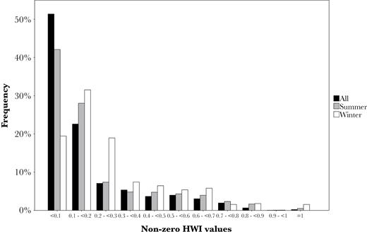
Distribution of non-zero half-weight index (HWI) values in the population using the full dataset and by season.

The SD and coefficient of variation (CV) of association indices were significantly higher in the real dataset than in the permuted data (real SD = 0.09, random SD = 0.05, P = 0.0001; real CV = 4.12; random CV = 2.59; P = 0.0001). Hence, we could reject the null hypothesis that individuals associated randomly. The social differentiation of the population was close to 1 (S ± SE = 0.98 ± 0.03), revealing a highly diverse range of associations within the population.

Hierarchical stratification

Applying the hierarchical dendogram display (cophenetic correlation coefficient [CCC] >0.8; Figure 2), social clusters diverged at an extremely low association index value (HWI of 0.02, maximum modularity of 0.68). The knot diagram presented an apparent constant rate of cumulative bifurcations, which only slightly increased at very low association indices. This pattern was still visible using a very restrictive association criterion (Supplementary Figure 3 in Supplementary Material S2). The network of associations was more interconnected at low HWI thresholds (Figure 3). However, without a larger number of strong bonds the network started to fragment very quickly when links were sequentially removed at low HWI thresholds. The network contained few stronger ties, as is visible when HWI = 0.5, with very small sets differentiated and individuals detached from the network. Associations in the Icelandic killer whale population did not appear to be clearly stratified into hierarchical tiers. Considering the wide range of association levels present, this does not mean that individuals only associate with a small set of companions.

Figure 2

Average-linkage cluster analysis. (a) Dendogram of 198 individuals encountered on at least 5 days (cophenetic correlation coefficient [CCC] = 0.94). (b) Knot diagram of cumulative number of bifurcations across HWI levels. (c) A maximum modularity-G, within hierarchical clustering, of 0.68 suggests a division into distinct clusters at an HWI of 0.02 (dashed line).

Figure 3

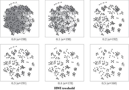
Network fragmentation with increasing HWI threshold. Isolated individuals are removed from the network (n indicates the number of individuals present). Note that at HWI >0.1 the network starts fragmenting quickly and more individuals become isolated from the network. Plotted using Fruchterman–Reingold force-directed layout (Fruchterman and Reingold 1991).

Examination of structure and movement pattern assortative mixing

Using Newman’s (2006) clustering technique, the population could be significantly divided in 18 distinct clusters (Table 2; Q = 0.66). The social clusters obtained in the analysis were of mixed sex–age classes. The cluster sizes varied between 3 and 33 individuals, with a mean ± SD of 11 ± 7.8 individuals per cluster. As expected, mean HWI within clusters was higher than between clusters (within clusters mean HWI ± SD = 0.27 ± 0.17 and maximum HWI ± SD = 0.65 ± 0.17; between clusters mean HWI ± SD = 0.01 ± 0.01 and maximum HWI ± SD = 0.01 ± 0.06). The assortativity coefficient of the network indicated some level of separation of associations according to movement pattern (including juveniles r ± SE = 0.44 ± 0.01; not including juveniles r ± SE = 0.49 ± 0.01) but much lower than would be expected if individuals favored associations with others of equal movement pattern and/or avoided associations with individuals with a different movement pattern. In fact, not all clusters were discriminated by movement pattern: 5 clusters were composed of a mix of individuals sighted in both seasons and individuals sighted in a single season.

Table 2

Summary of different clusters identified using Newman’s (2006) clustering technique

Cluster	n	Movement patterna	Days	Identificationsb	Mean HWI (SD)	Maximum HWI (SD)	S (SE)	S (SE) excluding juveniles
A	24 (5)	WB	34	2279	0.178 (0.04)	0.67 (0.15)	0.88 (0.1)	0.85 (0.1)
B	33 (3)	W	31	4112	0.12 (0.06)	0.62 (0.15)	1.01 (0.04)	1.01 (0.04)
C	9 (3)	B	15	798	0.54 (0.09)	0.73 (0.11)	0.08 (0.12)	0.05 (0.13)
D	11 (3)	B	60	3883	0.27 (0.06)	0.65 (0.13)	0.66 (0.06)	0.57 (0.08)
E	10 (4)	WB	24	549	0.2 (0.04)	0.55 (0.14)	0.96 (0.05)	0.86 (0.08)
F	3	B	10	91	0.12 (0.05)	0.18 (0)	0 (—)c	—
G	8 (4)	B	27	1918	0.49 (0.07)	0.67 (0.08)	0.17 (0.11)	0 (0.07)
H	13	B	31	1817	0.34 (0.04)	0.74 (0.07)	0.36 (0.12)	—
I	17 (4)	SB	65	2754	0.13 (0.05)	0.56 (0.19)	1.15 (0.03)	1.17 (0.04)
J	11 (3)	SB	33	1344	0.31 (0.16)	0.81 (0.25)	0.95 (0.06)	1.08 (0.05)
K	4 (1)	S	19	675	0.6 (0.08)	0.69 (0.08)	0 (0.11)	0 (0.03)
L	18 (5)	B	54	2825	0.16 (0.02)	0.59 (0.15)	1 (0.06)	0.91 (0.1)
M	4	B	8	142	0.27 (0.09)	0.5 (0.12)	0.47 (0.32)	—
N	7 (2)	SB	9	464	0.54 (0.08)	0.73 (0.1)	0 (0.19)	0 (0.12)
O	5	B	8	456	0.6 (0.1)	0.74 (0.12)	0 (0.2)	—
P	5 (2)	B	22	680	0.53 (0.09)	0.68 (0.11)	0.17 (0.09)	0 (0.09)
Q	7 (1)	B	31	1137	0.37 (0.1)	0.75 (0.13)	0.67 (0.14)	0.68 (0.14)
R	9 (1)	B	18	511	0.28 (0.13)	0.64 (0.18)	0.79 (0.09)	0.86 (0.09)

n, number of members with number of juveniles in brackets; HWI, half-weight index of association; S, social differentiation; SD, standard deviation; SE, standard error. ^aMovement pattern of non-juvenile members: W—only seen in the winter, S—only seen in the summer, B—seen in both seasons, WB—seen only in the winter or in both seasons, SB—seen only in the summer or in both seasons. ^bTotal number of photographic records of identified individuals of each cluster. ^cThere was insufficient association data to calculate SE of S for cluster F.

Clusters were highly variable in their complexity (Table 2). There was a wide range of values of social differentiation by cluster (with juveniles mean ± SE = 0.52 ± 0.1, min–max: 0–1.15; without juveniles mean ± SE = 0.49 ± 0.1, min–max: 0–1.17). The Pearson’s correlation test showed that social differentiation was significantly correlated with unit size (with juveniles r = 0.68, P = 0.002; without juveniles r = 0.62, P = 0.006). Within larger clusters not all associations were strong (representing high social preference) or weak, and members associated at many different degrees. In general, only a few individuals within each cluster maintained strong associations (>0.5 or >0.8) with other members and only 5 clusters had a mean HWI >0.5. From the measures of social structure, inspection of photographs and direct observations we concluded that we were not able to identify all companions of the members of cluster F. This cluster was most likely incomplete and therefore was not included in further descriptions.

Our analysis distinguished 3 types of social clusters in the population: stable (C, G, K, N, O, and P; Figure 4, Table 2), intermediate complexity (D, H, M, Q, and R; Figure 5, Table 2) and complex (A, B, E, I, J, and L; Figure 6, Table 2) clusters. Stable clusters had high mean HWI values, very low social differentiation and members with equal movement pattern (Figure 4, Table 2). Only in cluster G, 2 juveniles were subclustered with a very low modularity value, likely because they were born during the study period and only identified later in the study. Therefore, these clusters had no apparent substructuring and associations between members were generally more homogeneous but not equal.

Figure 4

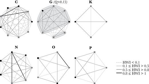
Sociogram of stable clusters. The thickness of the edges is related to the HWI value of association. Nodes represent individuals and are shaped/colored based on age–sex class (black circle: Adult female; gray circle: Adult male; black square: Other; gray square: Juvenile). There was no apparent subcluster division. Two juveniles were subclustered in cluster G but with a very low modularity value (Q), likely because the juveniles were only identified on the later years of the study, contrary to other members.

Figure 5

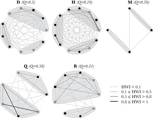
Sociogram of intermediate complexity clusters. The thickness of the edges is related to the HWI value of association. Nodes represent individuals and are shaped/colored based on age–sex class (black circle: Adult female; gray circle: Adult male; black square: Other; gray square: Juvenile). Q indicates the modularity of potential subcluster division.

Figure 6

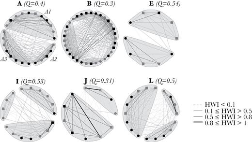
Sociogram of complex clusters. The thickness of the edges is related to the HWI value of association. Nodes represent individuals and are shaped/colored based on age–sex class (black circle: Adult female; gray circle: Adult male; black square: Other; gray square: Juvenile). Q indicates the modularity of potential subcluster division. A1, A2, and A3 indicate the 3 subclusters of cluster A.

Intermediate complexity clusters had intermediate values of mean HWI and social differentiation, showing potential but unclear subclustering (Q values generally <0.3), since individuals across potential subclusters also associated very frequently (Figure 5, Table 2). In general, cluster members had equal movement patterns, except for one cluster.

Complex clusters had very high values of social differentiation and very low mean HWI, but high maximum HWI (Table 2). In general, cluster members had different movement patterns, except for 2 clusters. Complex clusters showed potential substructuring (Figure 6), although this was not clear for all clusters (Q values of about 0.3 for cluster B and J). Associations between members of complex clusters were diverse and only some members maintained strong associations, with most associations being lower and at varying levels.

Temporal patterns of associations

The standardized lagged association rate SLAR $(g\text{'}\left(\tau \right))$ remained higher than would be expected from random associations over the investigated time periods (τ; Figure 7), indicating that nonrandom associations persisted over time.

Figure 7

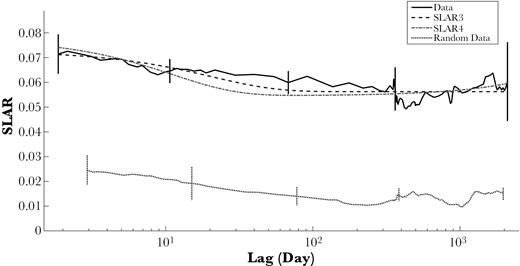
Standardized random and lagged association rates (SLAR, curve smoothed with 30000 moving average). Vertical bars represent temporal jackknife standard errors. The 2 models of the exponential family with the lowest QAIC values, SLAR3 and SLAR4, are shown (see Supplementary Material S4 for formulas and QAIC values).

The 2 more complex models presented a reasonable fit to the data (see Supplementary Material S4). The model SLAR3, labelled as “constant companions plus casual acquaintances” in Whitehead (2008a), had the lowest QAIC value, fitting the data best. Adding a second level of dissociation (SLAR4), gave a similar curve and a very small difference of QAIC to SLAR3 indicating some support for this model. However, contrary to SLAR3, there was no convergence and stable fit of SLAR4 when varying the parameters start values, which raised doubt on the suitability of this model for the data. For this reason the simpler model SLAR3, which has lowest QAIC and consistent parameters, was chosen to describe the temporal patterning of associations. This model indicated that the population was driven by a combination of longer-term relationships that last for many years, and temporary associations: $g\text{'}\left(t\right)=0.06+0.02e^{-0.0486t}.$ Temporary associations decayed exponentially, with the model suggesting important dissociations over scales of about 21 days (0.0486/days, SE = 0.09). The proportion of long-term associations was 77%, with only 23% of temporary relationships. This model’s fit estimated a typical group size of 14.8 individuals (SE = 2.5) and a typical unit size of 11.7 individuals (SE = 3.4).

Sex differences in association patterns

125 adults of known sex seen on 5 or more days were used in this analysis. Association levels within and between adult sex classes were similar, with low mean association indices and high maximum association indices (Table 3). The Mantel test did not reveal clear significant differences in association between, relative to within adult sex classes (permutation test, P = 0.05). If the analysis was restricted to 75 adults of know sex seen on more than 10 days there was no significant difference in association (permutation test, P = 0.13). The temporal analysis suggests that Female–Male, Male–Male, and Female–Female associations were somewhat stable across time and remained higher than random (Figure 8). For all types of associations, the SLAR was higher than the SLAR between all individuals (higher probability of association). In general, all SLAR were relatively stable over time and no sex difference was noticeable.

Table 3

Distribution of HWI for adult individuals seen at least 5 times, between and within sex classes.

Adult sex classes	Mean HWI (SD)	Maximum HWI (SD)
Females–All	0.02 (0.01)	0.59 (0.18)
Males–All	0.02 (0.01)	0.62 (0.21)
Females–Females	0.02 (0.01)	0.44 (0.21)
Females–Males	0.02 (0.01)	0.48 (0.24)
Males–Females	0.02 (0.01)	0.56 (0.23)
Males–Males	0.02 (0.01)	0.48 (0.26)
Within classes	0.02 (0.01)	0.46 (0.24)
Between classes	0.02 (0.01)	0.52 (0.23)
All–All	0.02 (0.01)	0.6 (0.19)

HWI, half-weight index of association; SD, standard deviation.

Figure 8

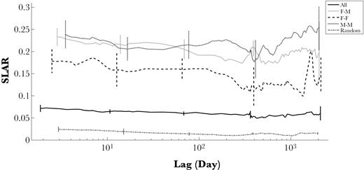
Standardized lagged association rates (SLAR) for different associations between adults. A different moving average was chosen accordingly to smooth lines. Jackknife grouping factor of 15, shown as vertical bars. SLAR between Females and Males (F–M) and between Males and Males (M–M) are high and relatively stable. Although lower, SLAR between Females and Females (F–F) are also high and much higher than the SLAR between all individuals (All) or if individuals had a random chance of associating (Random).

Adult female-specific analysis

32 adult females were sighted on more than 10 days over at least 3 years and only 12 of those were sighted on at least 20 days over at least 3 different years (Table 4). On both restriction conditions, associations were nonrandom (32 females: real SD = 0.11, random SD = 0.08, P = 0.0001 and real CV = 2.33, random CV = 1.72, P = 0.0001; 12 females: real SD = 0.17, random SD = 0.14, P = 0.0001 and real CV = 1.51, random CV = 1.31, P < 0.0001). The classical hierarchical clustering technique displayed dendograms with a varying level of associations between females, with significant clusters discriminated at low HWI values (see Table 4 and Supplementary Material S5). Although the cluster discrimination occurs at a higher HWI value for the set of females with the more restrictive observational threshold, it is still a low value and mostly weak associations are present within the discriminated clusters. The sociogram showed that, regardless of the observational threshold, associations between females are mainly weak even between most females from the same cluster (Figure 9). Also, there are several weak associations between females from many different clusters.

Table 4

Summary of the results of the adult female-specific analysis under 2 different observational thresholds

Observational threshold	>10 days, ≥3 years	≥20 days, ≥3 years
n	32	12
Mean ± SD sightings	19.1 ± 6.6 days (range of 11–34 days), over 4.6 ± 1 years (range of 3–6 years)	26.3 ± 4.5 days (range of 20–34 days), over 5.3 ± 0.5 years (from 5–6 years)
Nonrandom associations?	Yes	Yes
Dendogram	Supplementary Figure 10—Supplementary Material S5	Supplementary Figure 11—Supplementary Material S5
Divergence of clusters at HWI	0.04	0.21
Modularity	0.48	0.39

HWI, half-weight index of association; n, number of adult females in the analysis; SD, standard deviation.

Figure 9

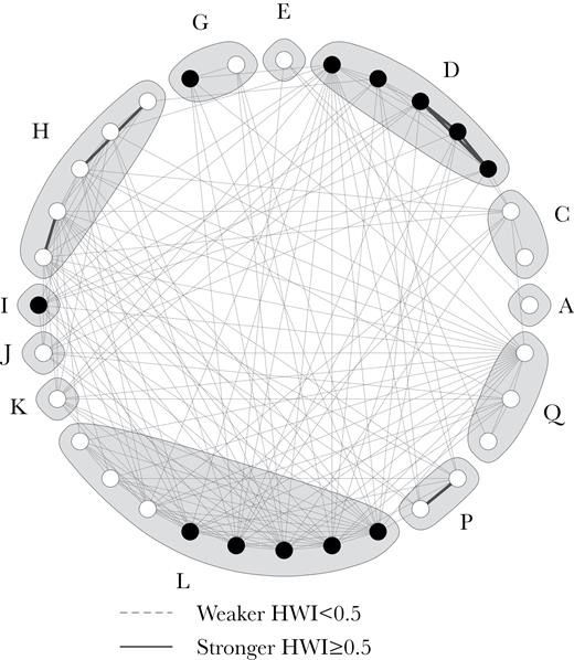
Sociograms of associations for the 32 most frequently encountered adult females (on more than 10 days over at least 3 years) from 12 different clusters. Nodes represent each female and are colored black if the individual was also seen on at least 20 days over at least 3 different years. Members of the same cluster were included within the same gray shading. Note the lack of strong associations and that there are many weak associations between females from different clusters. This is observed regardless of the minimum number of sightings, with predominantly weak associations across black nodes.

DISCUSSION

Our results showed that associations within the Icelandic population of herring-eating killer whales were non-random but the number of strong associations was small. Although the dendogram display of associations presented a high cophenetic correlation coefficient, social clusters were differentiated at extremely low levels of association. With this technique, individuals were clustered together also by least preferred associations, that is, weaker associations at very low HWI values, since not all individuals associated strongly within social units.

In a hierarchically structured society, transitions between structural tiers are clear because individuals within a social cluster (nested in a tier) associate more strongly than individuals within clusters at the level above. Societies without hierarchical nesting can still display a dendogram with a cophenetic correlation coefficient >0.8, indicating an acceptable match to the matrix of association indices (Bridge 1993), while being an inappropriate way of realistically displaying associations (Whitehead 2008a; Whitehead 2009). When individuals associate weakly overall the degree of potential hierarchical stratification is limited since an individual cannot represent its social unit because associations within a social unit are not equally strong. Our study showed this to be the case in this population. Thus, a non-stratified way of studying the society was considered more appropriate than techniques that assume a hierarchically organized social structure.

The population could be significantly divided into social clusters, which were highly diverse in complexity (even when using a more restrictive observation threshold; Supplementary Material S3—Supplementary Figure 10). A small portion of the clusters presented more coherent associations between members, which might represent cohesive basic structures. The majority of the clusters presented diverse association strengths and potential further subclustering. In some social clusters, many individuals did not strongly associate with all other members. This population presented both constant and temporary associations, not completely assorted by movement pattern and with no clear differences between sexes. Together these results suggest that the Icelandic herring-eating killer whale population has a multilevel society with no clear nested hierarchical structure of coherent social units, different from other populations of killer whales studied to date.

The evidence for nonrandom associations indicates that our results were not merely a consequence of the quality or constraints of the dataset. It is possible that some of the HWI values were negatively biased due to incomplete photographic coverage of groupings/aggregations (Ottensmeyer and Whitehead 2003). However, this type of bias would only increase the probability of not rejecting the null hypothesis of associations being random. The analysis using the most encountered adult females aimed at reducing the potential influence of recording sporadic associations, due to the observation that adult female resident killer whales have lower levels of mixing with other groups than other age–sex classes. Thus, a matrilineal structure may have been more clearly detectable among adult females than in the overall population. However, our population-level results were instead strongly supported by the adult female-specific analysis, with adult females also presenting an unclear hierarchical structure but a complex sociality with rare strong associations and many weak associations between females from the same cluster, and several associations between females from different clusters. There are indications that the weakness of associations is due to a high variability across years (associations on 1 year might not occur in a different year) but the small yearly number of sightings limits our ability to reach a definitive conclusion on the stability of associations and yearly preferences between these individuals.

A complex multilevel society

In the Icelandic herring-eating killer whale population individuals clearly associated at different levels, in some cases forming subcluster units. This society appears to tend towards an incompletely nested multilevel society (as in Figure 6 in de Silva and Wittemyer 2012). The levels of social stratification are not hierarchically distinct because transitions between levels are gradual and may vary among individuals or sets of individuals, i.e. not all individuals associate at similarly higher levels within social units and at distinctly lower levels between social units. The variability in cluster complexity indicates diverse association patterns among individuals and suggests different association strategies within the population.

Killer whale movement patterns did not assort their associations. In fact, individuals from different subclusters and clusters with markedly different movement patterns were commonly seen in tight groupings within less than 1 body length, a measure commonly used in other killer whale social structure studies to define a group (e.g., Ivkovich et al. 2010, Esteban et al. 2016; Figure 10). Furthermore, complex cluster A (Figure 6) was formed by 3 highly distinctive subclusters: subcluster A1, composed of individuals seen in Iceland year-round following the movements of the ISS herring stock; subcluster A2 composed of individuals that are only seen in Iceland in the winter; subcluster A3, composed of 5 individuals matched to the Scottish population (only 2 Others and 1 Juvenile from this subcluster were not matched) and sighted in Scotland in the summer (Samarra and Foote 2015). Combining social structure analysis with genetics could help to clarify the underlying aspects of social contact reported here between whales with different movement patterns and potentially different feeding ecologies in Iceland. It is worth noting that the individuals matched to the Scottish population were not always sighted together in Scotland (Samarra and Foote 2015) nor in Iceland. It is possible that individuals were missed in Scotland due to the opportunistic nature of data collection. However, in our study we could confirm that these individuals were not always associating at close proximity.

Figure 10

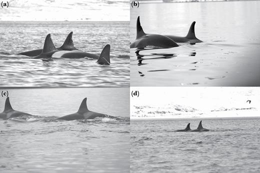
Examples of close associations between individuals from different subclusters and clusters: (a) IF-4 (Adult female, subcluster A3, Scotland ID 21) in close association with IS121 (Other, subcluster A1); (b) 997 (Adult female, subcluster A3, Scotland ID 19) in close association with IS041 (Adult female, cluster L); (c) IS172 (Other, subcluster A3) associating with IS049 (Adult female, cluster D); (d) IS229 (Other, subcluster A3) associating with IS030 (Adult female, cluster D).

The Icelandic multilevel society seems to be driven by a mix of both constant and temporary associations of mean duration of about 21 days. This temporal pattern of fission–fusion dynamics can occur in several types of social systems: 1) one in which constant permanent social units temporarily associate; 2) one in which individuals temporarily maintain casual but preferred associations; and 3) one in which permanent units exist but some individuals are “floaters” who move between units (Whitehead 2008a). When full units of individuals collectively join, the typical group size should be twice the typical unit size, as in Pacific sperm whales representing 2 temporal stable units joining (Whitehead et al. 1991) or larger, as in Nova Scotia long-finned pilot whales where a group is comprised of several units (Ottensmeyer and Whitehead 2003). Our study suggests that the temporal pattern did not result from permanent social units temporarily associating since the estimated typical group size was less than double of the typical unit size. Also, there was no indication of “floaters” moving between units and no evidence of adult dispersal in the Icelandic population. Instead, temporary associations are probably formed between preferred but casual associates or potentially by small sets of associates who temporarily associate with full permanent units, as small sets of associated “floaters”. Cluster members with weaker ties might represent these casual but preferred temporary associates. It is unknown if this behavioral flexibility is only maintained when killer whales aggregate in herring grounds or if it is seasonally shaped, so further studies will be necessary to understand this type of affiliation.

How can local ecological context shape killer whale social structure?

Methodological differences among studies (e.g., disparity in sampling procedures, definition of association, association index used) prevent a quantitative comparison of social structure between the Icelandic and other killer whale populations. Nevertheless, overall social structure comparisons can still be made. If sociality was determined by fish- versus mammal-eating ecological differences alone (Beck et al. 2012), we would expect that the Icelandic population would have a similar social structure to fish-eating resident killer whales. Indeed, mammal-eating killer whales show dispersal of either sex from maternal groups and relatively rare and unstable associations between adult males (Baird and Whitehead 2000) which we did not observe in our study and is also not present in residents (Bigg et al. 1990). These specific characteristics of the mammal-eating population are linked to optimal foraging group size adjustment when feeding on seals (Baird and Dill 1996). However, the clear stable matrilineal units (cohesive long-term groups) with members associating strongly and permanently (Bigg et al. 1990; Baird and Whitehead 2000) common to both mammal-eating and residents, was not found in the Icelandic herring-eating population.

Coherent basic social units have been described for other killer whale populations regardless of targeted prey (in Alaska: Matkin et al. 1999; Marion Island: Tosh et al. 2008; Northwest Pacific: Ivkovich et al. 2010; and Gibraltar: Esteban et al. 2016) and it has been considered a firm characteristic of the species despite ecological differences. In the Icelandic herring-eating population, the possible existence of matrilineal units is not clear, but cannot be rejected. For example, the potential subclustering of cluster D (Figure 5) is matched to direct observations of constant close proximity associates, which could be more similar to basic matrilineal units. Yet, these subclusters were still strongly associated and were seen frequently switching preference for close companions across days and years, as well as with individuals from other clusters. Therefore, if matrilineal units are present in this population it is possible that these are not entirely comparable to the ones present in other killer whale societies. An increase in the timespan of association data and genetic analysis, relating kinship and gene flow with the underlying patterns of associations, will be crucial to inform on the presence and characteristics of family bond-units in this population.

Further differences from the resident killer whale society were the lack of clear social tiers and hierarchical nesting in the Icelandic herring-eating society, which included fission–fusion dynamics at an individual (or sets of a few individuals) rather than at a group level (periodic merging of permanent social units). A parallel variation in multilevel structuring has been quantified in elephant societies (de Silva and Wittemyer 2012). African elephants (Loxodonta africana) maintain a clear multitiered society of coherent basic units that associate hierarchically. In contrast, Asian elephants (Elephas maximus) have a complex multilevel society without hierarchical structuring and nested units. Asian elephants do not maintain clear core groups and associations can be either ephemeral or long-term. de Silva and Wittemyer (2012) could not determine whether these differences were due to phylogenetic or ecological factors, but there were significant environmental differences between the 2 societies, such as differences in primary productivity and predation pressure.

Our study points to a different view of killer whale social structure, with a more dynamic and fluid sociality than generally inferred from broad ecology. As argued by Beck et al. (2012), ecology probably influences killer whale sociality rather than simply phylogenetic separation of populations. However, considering only fish- versus mammal-eating strategies as the ecological condition influencing sociality ignores important particularities of local ecological context. Herring-eating killer whales in Iceland target a prey with particular characteristics different from salmon and seals, such as antipredator behaviors, unpredictability and patchy distribution of high biomass. This shapes the feeding behavior of the population and probably its social structure.

Herring is a schooling fish with a diverse repertoire of antipredator maneuvers (Nøttestad and Axelsen 1999). Feeding upon this prey requires a highly coordinated group feeding technique to herd and catch herring (Similä and Ugarte 1993), unlike feeding techniques described for other fish-eating killer whale populations. To efficiently hunt larger concentrations or school sizes using a coordinated foraging technique, killer whales might benefit from larger group sizes to encircle the herring school (Vabø and Nøttestad 1997; Nøttestad et al. 2002). Active adjustment of killer whale numbers hunting herring schools has been observed in Norway (Nøttestad et al. 2002): on 4 observations of feeding groups (range of 22–46 individuals, mean ± SD = 33.5 ± 10.6 individuals), the 2 largest groups (38 and 46 individuals in total) occurred when the herring layer was larger (depth range of 150/160 m to 350 m) and were composed by different smaller groups of killer whales that gathered before starting to herd herring, arriving from different directions. In these conditions, it might be important to maintain a fission–fusion society where associations are flexible and individuals can actively adjust to these constantly changing requirements.

Herring can also undergo substantial changes in density and spatial distribution, particularly in overwintering grounds (Óskarsson et al. 2009). The unpredictability of the prey may additionally promote the maintenance of a more fluid and flexible sociality. A socioecological model proposed for dolphins suggests that when resources are unpredictable, dolphins will present wide range movements, reduced competition by cooperative foraging and larger groups to more effectively find and exploit large prey schools (Gowans et al. 2007). Dusky dolphins (Lagenorhynchus obscurus) in Argentina feed on schooling fish and present similar basic herding techniques to herring-eating killer whales (Würsig and Würsig 1980). Their target prey is also unpredictably distributed. The population presents a strong fission–fusion society with constantly fluctuating subgroup memberships (although some associations might be constant) that split for feeding and social purposes (Würsig and Würsig 1980; Würsig and Bastida 1986). This social structure is very different from dusky dolphins of New Zealand (Markowitz 2004), whose target preys are more predictable.

Finally, feeding aggregations in Iceland are very common during summer and winter, in grounds where herring are temporarily highly concentrated. The patchiness of a resource will influence whether animals do aggregate and, although these aggregations for feeding are not social structures (spatiotemporal clusters of individuals forced by nonsocial factors) they might act as catalysts for sociality (Whitehead 2008a). Recurring aggregations due to prey behavior may offer a special local ecological context for the establishment of associations, creating opportunities for social interactions with other individuals and somehow shaping the social structure of this population. The dynamic nature of the society described here may have been uncovered because our data collection took place mostly during periods when large aggregations of whales can occur, due to this particular ecological context. Future work focusing on social associations of herring-eating killer whales during periods when herring are more dispersed may reveal stronger social bonds, and clear long-term stable matrilineal groups, if group sizes are substantially lower than observed during the herring spawning and overwintering periods.

Other ecological differences such as habitat characteristics or historical capture might have also shaped the social structure of this population but we lack sufficient information to determine their influence at present. Furthermore, the Icelandic population is comprised of individuals with different seasonal movement patterns that associate at least seasonally. This alone can influence the social structure of the population, since different movement patterns within the same population suggest exposure to different environmental conditions. This might also lead to variation in social factors within the population, for example, mating competition or avoidance, which can influence the structuring of basic and high-order groups in mammals (Silk 2007). More information on the genetic relatedness of whales with different movement patterns is needed to understand how it may affect the resulting society.

We have shown that the Icelandic herring-eating killer whale population has a complex multilevel social structure with no clear hierarchical nesting and no strong social segregation by movement pattern. This social system appears to be different from other populations of killer whales worldwide, but continued photo-identification data will be crucial to investigate these questions over longer time scales and under different seasonal, spatial and prey behavioral contexts. The differences observed suggest that fish versus marine mammal prey-type alone does not define killer whale social structure and local ecological context, such as prey characteristics and foraging strategy, are probably strong drivers of sociality. The factors constraining hierarchical stratification of societies are little understood and to our knowledge are not addressed in socioecological frameworks (e.g., Emlen and Oring 1977; Wrangham 1980; Gowans et al. 2007). Comparative studies of populations targeting similar prey will be extremely important to quantitatively assess the degree of variation in multilevel social structuring with local ecological context.

SUPPLEMENTARY MATERIAL

Supplementary data are available at Behavioral Ecology online.

FUNDING

This work was supported by the Fundação para a Ciência e a Tecnologia (grant numbers SFSFRH/BD/30303/2006 and SFRH/BD/84714/2012); Icelandic Research Fund (i. Rannsóknasjóđur, grant number 120248402); National Geographic Society Science and Exploration Europe (grant number GEFNE65-12); Office of Naval Research (grant number N00014-08-10984); and a Russell Trust Award from the University of St. Andrews.

Data accessibility: Analyses reported in this article can be reproduced using the data provided by Tavares et al. (2016).

We would like to thank everyone that participated in the various field seasons, as well as Láki Tours for the opportunity to join their whale-watching trips, and the Vestmannaeyjar Research Centre, particularly Páll Jónsson, for logistical support. We thank Dr Volker Deecke for providing a platform for data collection in the summers of 2010 and 2015. We are grateful to Graeme Ellis for invaluable advice and useful discussions on killer whale social structure. We would also like to thank Dr Gísli Víkingsson and Dr Andrew Foote for providing the preliminary Icelandic photo-id catalogue. Field methods, designed for minimum distress to the animals, were approved by the School of Biology Ethics Committee of the University of St Andrews. All field research was carried out in compliance with local regulations and under permits provided by the Ministry of Fisheries. This manuscript benefited from the helpful comments of 2 anonymous reviewers.

Author notes

Address correspondence to S.B. Tavares, Sea Mammal Research Unit, School of Biology, University of St Andrews, Bute Building, St Andrews KY16 9TS, UK. E-mail:

Handling editor: Louise Barrett