


Abstract
In this study, we introduce an interpretable graph-based deep learning prediction model, AttentionSiteDTI, which utilizes protein binding sites along with a self-attention mechanism to address the problem of drug–target interaction prediction. Our proposed model is inspired by sentence classification models in the field of Natural Language Processing, where the drug–target complex is treated as a sentence with relational meaning between its biochemical entities a.k.a. protein pockets and drug molecule. AttentionSiteDTI enables interpretability by identifying the protein binding sites that contribute the most toward the drug–target interaction. Results on three benchmark datasets show improved performance compared with the current state-of-the-art models. More significantly, unlike previous studies, our model shows superior performance, when tested on new proteins (i.e. high generalizability). Through multidisciplinary collaboration, we further experimentally evaluate the practical potential of our proposed approach. To achieve this, we first computationally predict the binding interactions between some candidate compounds and a target protein, then experimentally validate the binding interactions for these pairs in the laboratory. The high agreement between the computationally predicted and experimentally observed (measured) drug–target interactions illustrates the potential of our method as an effective pre-screening tool in drug repurposing applications.
Introduction
Drug–target interaction (DTI) characterizes the binding between a drug and its target, critical to the discovery of novel drugs and repurposing of existing drugs. High-throughput screening remains the most reliable approach to examining the affinity of a drug toward its targets. However, the experimental characterization of every possible compound–protein pair quickly becomes impractical due to the immense space of chemical compounds, targets and mixtures. This motivates the use of computational approaches for DTI prediction. Molecular simulation and molecular docking are among the earlier computational approaches, which typically require 3D structures of the target proteins to assess the DTI. The application of these structure-based methods is limited, as there are many proteins with unknown 3D structures, and they involve an expensive process. Machine Learning (ML) algorithms have emerged to overcome some of these challenges in the process of drug design and discovery. Traditional shallow ML-based models, such as KronRLS [1] and SimBoost [2], require hand-crafted features, which highly affect the performance of the models. Deep Learning has advanced these traditional models due to their ability to automatically capture useful latent features, leading to highly flexible models with extensive power in identifying, processing and extrapolating complex patterns in molecular data. Deep Learning models for DTI can be mainly categorized into two classes. One class is designed to work with sequence-based input data representation. Examples of this type include convolutional neural networks (CNNs) and recurrent neural networks (RNNs). These models are incapable of capturing structural information of the molecules, leading to the degraded predictive power. This limitation motivates the use of a more natural representation of molecules and the introduction of a second class of Deep Learning models, namely graph neural networks (GNNs). GNNs use graph descriptions of molecules, where atoms and chemical bonds correspond to nodes and edges, respectively. Graph convolutional neural network (GCNN) and graph attention network (GAT) [3] are the two widely used GNN-based models in computer-aided drug design, and discovery [4–6]. All these graph-based models use amino acid sequence representations for proteins, which cannot capture the 3D structural features that are key factors in the prediction of DTIs. Obtaining the high-resolution 3D structure of the proteins is a challenging task, besides the fact that proteins contain a large number of atoms requiring a large-scale 3D (sparse) matrix to capture the whole structure. To alleviate this issue, an alternative strategy has been adopted wherein the proteins are represented by a 2D contact (or distance) map that shows the interaction of proteins’ residue pairs in the form of a matrix [7, 8]. It is worth mentioning that a contact (or distance) map is typically the output of protein structure prediction, which is based on heuristics and provides only an approximation abstraction of the real structure of the protein; generally, different from the one determined experimentally via X-ray crystallography or by nucleic magnetic resonance spectroscopy (NMR) [9]. Taken all together, and considering the fact that the binding of a protein to many molecules occurs at different binding pockets rather than the whole protein, in this paper, we propose AttentionSiteDTI, a graph-based deep learning model that incorporates structural features of small molecules and proteins’ binding sites in the form of graphs into the pipeline of DTI prediction task. The structural features of small molecules and proteins, which are automatically learned by the model, will be more conducive to downstream tasks. Our approach is inspired by models developed for sentence classification in the field of Natural Language Processing (NLP) and is motivated by the fact that the structure of the drug–target complex can be very similar to the structure of a natural language sentence in that the structural and relational information of the entities is key to understanding the most important information of the sentence. In this regard, each protein pocket or drug is analogous to a word, and each drug–target pair is analogous to a sentence. Our AttentionSiteDTI, which utilizes a self-attention bidirectional Long Short-Term Memory (LSTM) mechanism, is highly explainable due to its self-attention. In essence, self-attention provides an understanding of which parts of the protein are most probable to bind with a given drug. Visualization of the proposed framework can be found in Figure 1. As the computational results show, our model outperforms many state-of-the-art models in terms of multiple evaluation metrics. The results of our ablation study show that the attention mechanism is very effective in capturing important factors governing DTI. Also, our in-lab experimental validation shows high agreement between computationally predicted and experimentally observed binding interaction between seven candidate compounds and spike (or ACE2) protein.
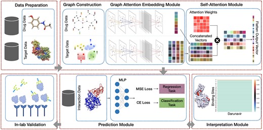
Our proposed framework includes five main modules: (1) Preprocessing module that consists of finding the binding sites of proteins; (2) AttentionSiteDTI deep learning module, where we construct graph representations of ligands’ SMILE and proteins’ binding sites, and we create a graph convolutional neural network armed with an attention pooling mechanism to extract learnable embeddings from graphs, as well as a self-attention mechanism to learn relationship between ligands and proteins’ binding sites; (3) Prediction module to predict unknown interaction in a drug–target pair, which can address both classification and regression tasks; (4) Interpretation module to provide a deeper understanding of which binding sites of a target protein are more probable to bind with a given ligand. (5) In-lab validations, where we compare our computationally predicted results with experimentally observed (measured) drug–target interactions in the laboratory to test and validate the practical potential of our proposed model.
Contribution
The main contributions of our study are summarized as follows.
We propose a novel formulation of DTI prediction problem inspired by recent developments in NLP that achieves state-of-the-art performance while exhibiting high generalizability and interpretability. Our approach is analogous to the sentence classification problem in NLP, where the drug–target complex is treated as a sentence with relational meaning between its biochemical entities a.k.a. protein pockets and drug molecule. We solve our sentence classification problem using an end-to-end GCNN-based model, which enables simultaneous learning of (1) context-sensitive embeddings from the graphs of molecules and protein pockets (that is, the embeddings are not fixed, but they change according to the context (i.e. sentence) in which they appear), and (2) a prediction model to capture the most important contextual semantic or relational information in a biochemical sequence (drug–target complex) for relation classification similar to sentence classification in NLP. Details of our GCNN-based model can be found in subsection Graph Attention Embedding Module.
Our proposed model is highly generalizable due to our target protein input representation that uses protein pockets encoded as graphs. This helps the model concentrate on learning generic topological features from protein pockets, which can be generalized to new proteins that are not similar to the ones in the training data. Generalizability of our model is specifically showcased by its superior performance on unseen proteins in BindingDB dataset (Figure 4). Data Preparation and Graph Construction subsections discuss the details on how we prepare and use protein inputs for our model.
Our proposed model is the first to be interpretable using the language of protein binding sites. This is important because it will help drug designers identify critical protein sites along with their functional properties. This is achieved by devising a self-attention mechanism, which makes the model learn which parts of the protein interact with the ligand, while achieving state-of-the-art prediction performance. Self-Attention subsection explains how the mechanism works by selectively focusing on the most relevant parts of the inputs.
Finally, we validate the practical potential of our model in the prediction of binding interactions in real-world applications. We conduct in-lab experiments to measure the binding interaction between several compounds and Spike (or ACE2) protein, and compare the computationally predicted results against the ones experimentally observed in the laboratory. In-Lab Validation section provides the details of our in-lab experiments.
Related work
Deep learning-based approaches have been successfully deployed to address the problem of DTI prediction. The main difference between deep learning approaches is in their architecture as well as the representation of the input data. As previously mentioned, small molecules of the drugs can be easily and effectively represented in one-dimensional space, but proteins are much bigger molecules with complex interactions, and 1D representations can be insufficient. Although the datasets containing the 3D structure of the protein are limited, some recent deep learning-based literature has used them in their study. For example, AtomNet [10], is the first study that used the 3D structure of the protein as input to a 3D CNN to predict the binding of drug–target pairs using a binary classifier. Ragoza et al. [11] proposed a CNN scoring function that took the 3D representation of the protein–ligand complex and learned the features critical in binding prediction. This model outperformed the AutoDock Vina score in terms of discriminating and ranking the binding poses. Pafnucy[12] is a 3D CNNs that predicted the binding affinity values for the drug–target pairs. This study represented the input with a 3D grid and considered both proteins and ligands atoms similar. Using a regularization technique, their designed network focused on capturing the general properties of interactions between proteins and ligands.
There are limitations associated with all these studies. For example, it is a highly challenging task to experimentally obtain a high-quality 3D structure of proteins, which explains why the number of datasets with 3D structure information is very limited [8]. Most studies that use 3D structural information utilize CNNs, which are sensitive to different orientations of the 3D structure, besides the fact that these approaches are computationally expensive. To overcome these limitations, recent studies such as done in [13–15] have proposed graph convolutional network approaches, which take 3D structure of proteins as input for DTI prediction task. There are other studies that applied GCNN to the 3D structure of the protein–ligand complex. Among these studies, GraphBAR [6] is the first 3D graph CNN that used a regression approach to predicts drug–target binding affinities. They used graphs to represent the complex of protein–ligand instead of 3D voxelized grid cube. These graphs were in the form of multiple adjacency matrices in which the entries were calculated based on distance and feature matrices of molecular properties of the atoms. Also, they used a docking simulation method to augment additional data to their model. Lim et al. [5] proposed a graph convolutional network model along with a distance-aware graph attention mechanism to extract features of the interactions binding pose directly from the 3D structure of drug–target complexes from docking software. Their model improved over docking and several deep learning-based models in terms of virtual screening and pose prediction tasks. However, their approach had limitations such as less explainability as well as additional docking errors added to the deep learning model. Pocket Feature is an unsupervised autoencoder model, which was proposed by Torng et al. [4], to learn representations from binding sites of the target proteins. The model used 3D graph representations for protein pockets along with 2D graph representations for drugs. They trained a GCNN model to extract features from the graphs of protein pockets and drugs’ SMILEs. Their model outperformed 3DCNN, as was done in [11] and docking simulation models such as AutoDock Vina [16], RF-Score [17] and NNScore [17]. Zheng et al. [8] pointed out the low efficiency of using direct input of three-dimensional structure and utilized a 2D distance map to represent the proteins. They further converted the problem of DTI prediction into a classical visual question and answering (VQA) problem, wherein, given a distance map of a protein, the question was whether or not a given drug interacts with the target protein. Although their model outperformed several state-of-the-art models, their VQA system is able to solve a classification task only, where it predicts if there is an interaction between drug–target pairs.
Materials and Methods
Overview
We introduce an end-to-end graph-based deep learning framework, AttentionSiteDTI, to address the problem of DTI prediction. We consider the DTI prediction task as a binary classification problem. The aim is to learn a predictive function |$\gamma (.)$|, with graph inputs of drugs and proteins, to output binary predictions suggesting the occurrence or absence of interactions. The overall architecture of AttentionSiteDTI is shown in Figure 1. It consists of four modules: data preparation, graph embedding learning module, prediction module and interpretation module. In the data preparation, we find the binding sites of the proteins using the algorithm proposed in [18]. In the next step, the graphs of protein pockets and ligands are constructed and fed into a graph CNN to learn the embeddings from the corresponding graphs. Feature vectors of drug and protein are then integrated to obtain drug–target complex representation that incorporates their structural features. The concatenated representations are then fed into a binary classifier for predicting DTIs. The self-attention mechanism in the network uses concatenated embeddings of drug–target pairs as input to compute the attention output, which enables interpretability by making the model learn which parts of the protein interact with the ligand in a given drug–target pair.
Data Preparation
We use the 3D structure of the proteins that are extracted from Protein Data Bank (PDB) files of proteins. PDB data are collections of submitted experimental values (e.g. from NMR, x-ray diffraction, cryo-electron microscopy) for proteins. In order to find the binding sites of the proteins, we use the algorithm proposed by Saberi Fathi et al. [18], which is one of the simplest methods to extract the binding sites of a protein from its 3D structure. This method is a simulation-based model, and it can be utilized prior to feeding the data into an end-to-end architecture, which helps reduce the model’s complexity. As shown in [18], despite the simplicity of this model, its performance is comparable to other simulation-based methods with higher complexity.
This algorithm computes bounding box coordinates for each binding site of a protein. These coordinates are then used to reduce the complete protein structure into a subset of peptide fragments. Figure 2 provides a visualization of a protein’s binding sites extracted using the algorithm in [18].
![Depiction of COVID spike protein and ACE2 complex with PDB-ID of 6M0J; Color of the surface represents the binding sites computed through Saberi Fathi et al. algorithm. These binding sites are used to create the input to our graph embedding learning module. All protein visualization was produced with UCSF Chimera software [19].](https://oup.silverchair-cdn.com/oup/backfile/Content_public/Journal/bib/23/4/10.1093_bib_bbac272/1/m_bbac272f2.jpeg?Expires=1716356161&Signature=iSKTzUr5ITxKK894LZ0zLaUUm0bxXfobNTlr9NbTPO7nHqJQFfx68cYAbZGRbnkEsx6bYR9Iym1MlSrXPWjqJm0ZpC4fefC0uOMx75XUazj9Y1PkxShDF9N72eAZACgFtzKW-dK074LPBsmm-n3VqHgnYnA4xYguOcNKM~MmD6AhTi0EgMPQxgzTHt1x1eAXQrBaKbFBDTjXdJwJkei-DCxRaDsyrDTO2~Ya2XZmabR1eSgEMu9n~otdYIU4O-1uTnPsi4dAbMsHjRyVVQPwzXtC7EjJpWKWLpDeJ-hKZnBOmTmcpVAJok8Zz0-PhUskGnJe9bGX3GB5uJv~Mi1zCQ__&Key-Pair-Id=APKAIE5G5CRDK6RD3PGA)
Depiction of COVID spike protein and ACE2 complex with PDB-ID of 6M0J; Color of the surface represents the binding sites computed through Saberi Fathi et al. algorithm. These binding sites are used to create the input to our graph embedding learning module. All protein visualization was produced with UCSF Chimera software [19].
Graph Construction
Protein
Following the extraction of a protein’s binding sites, we then represent them as individual graphs wherein each atom is a node, and the connections between atoms are the edges in the graph. One-hot encoding of the atom type, atom degree, the total number of hydrogen atoms (attached) as well as the implicit valence of the atom are used to compute the feature vector of each atom. This approach yields a vector with a size of |$1 \times 31$| for each node. These features are summarized in Table 1. Having multiple graphs, representing different binding pockets of a given protein, leads to the generation of multiple embeddings for that particular protein.
Encoding atom features in each extracted fragments
| Type | Encoding |
|---|---|
| Atom type | C, N, O, S, F, P, Cl, Br, B, H (onehot encoding) |
| Degree of atom | 0, 1, 2, 3, 4, 5, 6, 7, 8 (onehot encoding) |
| Number of hydrogen attached | 0, 1, 2, 3, 4 (onehot encoding) |
| Implicit valence electrons | 0, 1, 2, 3, 4, 5 (onehot encoding) |
| Is aromatic | 0, 1 (onehot encoding) |
Ligand
A bidirectional graph is constructed for each ligand, which is represented in Simplified molecular-input line-entry system (SMILE) format in DTI datasets. Note that in this study, hydrogen atoms are not explicitly represented as the nodes in the graph. Similarly, a vector is constructed to represent the atom’s features in the graph of ligand. More specifically, the one-hot encoding of the atom type, the atom degree, the formal charge of the atom, number of radical electrons of the atom, the atom’s hybridization, atom’s aromaticity and the number of total hydrogens of the atom are used to construct the features of the atoms in a ligand. This approach yields a vector with a size of |$1 \times 74$| for each node. Generated graphs for proteins and ligands are then fed into a GCNN to learn the corresponding embeddings.
Graph Attention Embedding Module
Topology Adaptive Graph Convolutional Networks
Pooling Mechanism
Self-Attention Module
Sequence Handling
Self-Attention
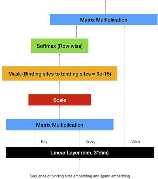
Self-Attention scaled dot product.
This self-attention mechanism uses a sequence of embeddings as input to extract Q, K and V. The attention output is then computed using Eq. 4.
Bi-LSTM
Long Short Term Memory (LSTM) is a variation of RNNs with memory cells, capable of learning long-term dependencies through the use of ‘additional gates’ incorporated in its architecture. Conventional LSTM only preserves information of the past, as the network receives the sequence inputs only in the original forward direction. Bidirectional LSTM networks add a second layer to LSTM networks to preserve the future and the past information by letting the sequence inputs flow in both forward and backward directions [23]. This feature of Bi-LSTM is especially useful in our particular application, as there is no meaningful order in which the protein binding sites and the ligand should interact. Thus, the future context in the sequence is as important as the past context. We use an element-wise sum to combine the outputs of the forward and backward passes.
Prediction Module
Classifier
The features previously computed are concatenated to a 1D vector |$I$|, which is then passed to the classification layers. In this study, two fully connected layers are used to map the extracted features into a final classification output. We use multilayer perceptron with Relu activation function. Also, dropout is used before each linear layer for better generalizability.
Experiments
Datasets
We demonstrate the merit of the proposed model via a series of comparative experiments. We compare our AttentionSiteDTI with several state-of-the-art methods using three benchmark datasets, which provide 3D structure information of target proteins, required by our model. These datasets include the DUD-E dataset, the Human dataset and the customized BindingDB dataset. Table 2 summarizes the statistical information of these datasets. We use a simple docking-based model, proposed in [18], to find the binding sites of the target proteins. It it worth mentioning that we expect a boost in the performance of our model with the use of a more advanced prediction/computation approach that is more accurate in finding binding sites of the proteins.
Description and statistics of the three benchmark datasets: DUD-E dataset, Human dataset and BindingDB dataset
| Datasets | Drugs | Proteins | DT pairs | Active | Inactive |
|---|---|---|---|---|---|
| DUD-E | 22 886 | 102 | 1429 790 | 22 645 | 1407 145 |
| Human | 2726 | 2001 | 6728 | 3364 | 3364 |
| Bindingdb | 989 383 | 8536 | 2286 319 | 39 747 | 31 218 |
| Datasets | Drugs | Proteins | DT pairs | Active | Inactive |
|---|---|---|---|---|---|
| DUD-E | 22 886 | 102 | 1429 790 | 22 645 | 1407 145 |
| Human | 2726 | 2001 | 6728 | 3364 | 3364 |
| Bindingdb | 989 383 | 8536 | 2286 319 | 39 747 | 31 218 |
DUD-E This dataset [25] consists of 102 targets from eight protein families. Each target has around 224 active compounds and more than 10 000 decoys, which were computationally generated in a way that their physical attributes are similar to active compounds but they are topologically dissimilar. Following the prior works by Ragoza et al. [11] and Zheng et al. [8], and in order to make a head-to-head comparison with the benchmark models, we performed 3-fold cross-validation in this dataset, and we reported the average performance on the evaluation metrics. Each fold was split based on the target in that similar targets were kept in the same fold. We used random undersampling on the decoys to make the training set balanced, and we used unbalanced test sets for evaluations.
Human This dataset was built by combining a set of highly credible and reliable negative drug–protein samples via a systematic in silico screening method with the known positive samples [26]. The dataset consists of 5423 interactions. For a head-to-head comparison, we used the same train, validation and test splits (80%,10%,10%) as were used in DrugVQA [8].
BindingDB This dataset [27] contains experimentally based assays of the interactions between small molecules and proteins. Following the work in DrugVQA [8], we used a small subset of the dataset, which consists of 39 747 positive and 31 218 negative samples. Further, in order to validate the generalization ability of our proposed model, the testing set was split into two groups of the proteins: those that are seen during the time of training versus those that are not being seen by the model.
Implementation and evaluation strategy
Experimentation strategies. We used Pytorch 1.8.2 (long-time support version) for our implementations. We trained the models with a batch size of 100 for 30 epochs, and we used Adam optimizer for training the network with a learning rate of 0.001. Also, for better generalization, a dropout with a probability of 0.3 was used before each fully connected layer. The GPU that we used for the experimentation was Nvidia RTX 3090 with 24 GB of memory. We used four as the number of hops in TAGCN for proteins and two for ligands. The size of the hidden state for the BiLSTM layer in our model was set to 31, which was the output of the graph convolution layer (TAGCN). We used padding of zero to reshape each matrix to the maximum number of binding pockets in the datasets. All hyperparameters were tuned to yield the best result for each dataset, which can be seen in Table 3. This hyperparameter tuning was performed by a simple grid search over a range of values, shown in Table 4
Dataset’s Training Hyperparameters (FC is representing number of fully connected layers, L-GCN and P-GCN are number of Graph convolutional layers for extracting ligands and protein binding sites embedding, respectively)
| Datasets | FC | L-GCN | P-GCN |
|---|---|---|---|
| DUD-E | 2 | 18 | 16 |
| Human | 6 | 4 | 3 |
| Bindingdb | 6 | 4 | 3 |
| Datasets | FC | L-GCN | P-GCN |
|---|---|---|---|
| DUD-E | 2 | 18 | 16 |
| Human | 6 | 4 | 3 |
| Bindingdb | 6 | 4 | 3 |
Grid search considered values for hyperparameter tuning
| TAGCN Hops | FC | L-GCN | P-GCN | LR | Dropout | batch size |
|---|---|---|---|---|---|---|
| |$\left [1-8\right ]$| | |$\left [1-8\right ]$| | |$\left [4-20\right ]$| | |$\left [4-20\right ]$| | |$\left [10^{-2}, 10^{-3},\right. \left. 10^{-4}, 10^{-5} \right ]$| | |$\left [0.1-0.6\right ]$| | |$\left [40, 60, 80,\right. \left. 100, 120\right ]$| |
The choice of different performance metrics as well as different benchmark models for different datasets is mainly for the head-to-head comparison with the results reported in the literature. Nevertheless, the reported metrics are the most widely used evaluation metrics in classification-based models in DTI literature [28]. Also, for comparison, we include a suit of different computational models including (a) traditional ML-based methods such as K-Nearest Neighbors (KNN), L2-logistic (L2), NN-score [29] and Random Forest-score (RF-score) [30]; (b) open-source molecular docking programs including AutoDock Vina [16] and Smina [31]; (c) string representation-based deep learning models such as AtomNet [10] and 3D-CNN [11]; and (d) graph representation-based deep learning models such as Graph CNNs(GCNs) [21], CPI-GNN [32], DrugVQA [8], TransformerCPI [33], PocketGCN [4], GNN [34] and GraphDTA [15] that have been developed to address the problem of DTI prediction.
Ablation Study Results
| Ablation tests | BindingDB | Human | DUD-E | |||
|---|---|---|---|---|---|---|
| AUC | ROC | AUC | ROC | AUC | ROC | |
| Bi-LSTM | 0.863 | 0.889 | 0.976 | 0.979 | 0.954 | 0.562 |
| Self-Attention | 0.940 | 0.981 | 0.991 | 0.990 | 0.961 | 0.602 |
| Bi-LSTM + Self-Attention | 0.925 | 0.973 | 0.984 | 0.982 | 0.971 | 0.623 |
Ablation study The ablation study illustrates the effectiveness of several text classification techniques in our proposed AttentionSiteDTI framework. We report the AUC and the ROC of all experiments, which is widely used in the literature. The results of this study can be found in Table 5, indicating that the attention mechanism is the most effective method in text classification, and it is particularly advantageous due to its power in explainability. The Bi-LSTM architecture cannot focus solely on interactions between ligand and binding sites; therefore, it has inferior results compared with other proposed architectures.
As the results show, the self-attention shows superior performance compared with Bi-LSTM+self-attention, except on the DUD-E dataset. This can be explained by the fact that DUD-E, in nature, is a more challenging dataset in the sense that DUD-E decoys (ligands with negative interactions) are matched to the physical chemistry of ligands with positive interactions (in terms of molecular weight, predicted logP, number of rotatable bonds and hydrogen bond donors and acceptors). Decoys should not truly bind to fulfill their duty as negative controls. Hence DUD-E employed 2D similarity fingerprints to reduce the topological similarity between decoys and ligands. In brief, DUD-E decoys were selected to physically mimic ligands with positive interactions (and hence to be difficult to dock), while they are also being topologically distinct to reduce the possibility of actual binding [25]. These decoys’ similarities are particularly challenging for approaches that utilizes ligands’ physical structure such as graph-based neural networks. To this end, a single attention module struggles to create features that are discriminating enough for the classifier head. Therefore, the additional use of a Bi-LSTM layer helps create richer features, which leads to the improved performance of the model on this challenging dataset. To be more specific, we achieved higher accuracy on the DUD-E dataset using an Bi-LSTM layer to capture the short-range relationships, followed by the self-attention mechanism to further improve the quality of the features. Since the other two datasets (Human and BindingDB) are not as challenging as the DUD-E dataset, adding a Bi-LSTM layer not only does not seem to be advantageous but it may also cause the model to overfit.
Comparison on the DUD-E dataset On DUD-E dataset, we compared our proposed model with several state-of-the-art models that can be divided into four categories: (1) ML-based methods such as NN-score [29], and Random Forest-score (RF-score) [30]; (2) open-source molecular docking programs including AutoDock Vina [16] and Smina [31]; (3) deep learning-based models such as AtomNet [10], 3D-CNN [11], which use neural networks to extract features from 3D structural information; and (4) graph-based models such as PocketGCN [4], GNN [34], DrugVQA [8], which are all based on graph representations. PocketGCN utilizes two Graph-CNNs that automatically extract features from the graph of protein pockets and ligands to capture protein–ligand binding interactions. CPI-GNN [32] is a prediction model that combines a graph neural network for ligands and a CNN for targets. DrugVQA utilizes a 2D distance map to represent proteins in a Visual Question Answering system, where the images are the distance maps of the proteins, the questions are the SMILES of the drugs and the answers are whether the drug–target pair will interact. Note that the scores of these models are collected from the work in [8]. Also, we employed the F1 score and ROC enrichment (RE) at thresholds 0.5%, 1%, 2% and 5%. As the results in Table 6 indicate, our model achieves state-of-the-art performance in DTI prediction on all metrics with significant improvement at 0.5% RE. Also, we hypothesize that the poor performance of AtomNet and 3D-CNN may be due to the sparsity of 3D space, as they use the whole 3D structure of the proteins.
DUD-E Dataset Comparison
| AUC | 0.5% RE | 1.0% RE | 2.0% RE | 5.0% RE | |
|---|---|---|---|---|---|
| NN Score | 0.584 | 4.166 | 2.980 | 2.460 | 1.891 |
| RF-score | 0.622 | 5.628 | 4.274 | 3.499 | 2.678 |
| Vina | 0.716 | 9.139 | 7.321 | 5.811 | 4.444 |
| Smina | 0.696 | - | - | - | - |
| 3D-CNN | 0.868 | 42.559 | 26.655 | 19.363 | 10.710 |
| AtomNet | 0.895 | - | - | - | - |
| PocketGCN | 0.886 | 44.406 | 29.748 | 19.408 | 10.735 |
| GNN | 0.940 | - | - | - | - |
| DrugVQA | 0.972 | 88.17 | 58.71 | 35.06 | 17.39 |
| AttentionSiteDTI | 0.971 | 101.74 | 59.92 | 35.07 | 16.74 |
Comparison on the human dataset On the Human dataset, we compared our model against several traditional ML models such as K-Nearest Neighbors (KNN), Random Forest (RF), L2-logistic (L2) (these results were gathered from [17]); and some recently developed graph-based approaches including Graph CNNs(GCNs) [21], CPI-GNN [32], DrugVQA [8], TransformerCPI [33] as well as GraphDTA [15]. GraphDTA was originally designed for regression task, and later was tailored to binary classification task by [35]. For a head-to-head comparison with other models, we followed the same experimental setting as in [34, 36]. Also, we repeated our experiments with three different random seeds, similar to DrugVQA [8]. The performances of the aforementioned models were obtained from [35], as summarized in Table 7. It can be observed that the prediction performance of our proposed model is superior to all ML- and GNN-based models, and it achieves competitive performance with DrugVQA in terms of precision and recall. The relatively low performance of ML-based models is indeed in line with our expectations and is due to their use of low-quality features, unable of capturing complex nonlinear relationships in DTI. The deep learning models, on the other hand, are very powerful in extracting important features governing the complex interactions in a drug–target pair. On this basis, our model further improves on the accuracy, indicating that the quality of learned information in DTIs is guaranteed by the back propagation of the end-to-end learning of our AttentionSiteDTI.
Human Dataset Comparison
| AUC | Precision | Recall | F1 Score | |
|---|---|---|---|---|
| K-NN | 0.86 | 0.798 | 0.927 | 0.858 |
| RF | 0.940 | 0.861 | 0.897 | 0.879 |
| L2 | 0.911 | 0.861 | 0.913 | 0.902 |
| SVM | 0.910 | 0.966 | 0.950 | 0.958 |
| GraphDTA | 0.960 | 0.882 | 0.912 | 0.897 |
| GCN | 0.956 | 0.862 | 0.928 | 0.894 |
| CPI-GNN | 0.970 | 0.923 | 0.918 | 0.920 |
| E2E/GO | 0.970 | 0.893 | 0.914 | 0.903 |
| DrugVQA | 0.979 | 0.954 | 0.961 | 0.957 |
| BridgeDPI | 0.990 | 0.963 | 0.949 | 0.956 |
| AttentionSiteDTI | 0.991 | 0.951 | 0.975 | 0.963 |
Comparison on the BindingDB dataset On BindingDB dataset, we further compared our model against Tiresias [37], DBN [38], CPI-GNN [32], E2E [39], DrugVQA [8] and Bridge-DPI [35] as baselines. Tiresias uses similarity measures of drug and target pairs. DBN uses stacked restricted Boltzmann machines with inputs in the form of extended connectivity fingerprints. As mentioned earlier, CPI-GNN combines a graph neural network for compounds and a CNN for targets to capture DTIs. E2E is a GNN-based model that uses LSTM to learn drug–target pair information with Gene Ontology annotations. DrugVQA, as previously mentioned, is a Visual Question Answering system, where the images are the distance maps of the proteins, the questions are the SMILES of the drugs and the answers are whether the drug–target pair will interact. Finally, BridgeDPI uses CNNs to obtain embeddings for drugs and proteins, as well as a GNN to learn the associations between proteins/drugs using some hyper-nodes that are connections between proteins/drugs.
Note that the scores for all these models were derived from [35]. Also, following suggestions from previous works, we report the prediction results in terms of AUC and Accuracy (ACC) on the test set, which is divided into a set of unseen proteins (the proteins that are not observed in the training set) and a set of seen protein (the proteins that are observed in the training set). This, indeed, makes the customized BindingDB dataset suitable to assess models’ generalization ability to unknown proteins, which should be the focus in prediction problems (i.e. cold-start problem), as there are a large number of unknown proteins in nature.
As experimental results indicate in Figure 4, all models generally perform well on seen proteins with AUC above 0.9 and ACC exceeding 0.85. However, these models show different and much worse performance on unseen proteins, which reflects the complexity of this more realistic learning scenario. Tiresias is a similarity-based model that uses a set of expert-designed similarity measures as the features for proteins and drugs. The poor performance of Tiresias on the unseen proteins is perhaps due to the fact that these handcrafted features are not sufficient in capturing interactions between drug–target pairs, thus resulting in the accuracy of even less than 0.5 on unseen proteins. On the other hand, the good performance of deep learning-based models, including DBN, CPI-GNN, E2E, DrugVQA, BridgeDPI, as well as our AttentionSiteDTI, shows the effectiveness of these models in capturing relevant features that are critical in DTI prediction problem. As the results show, our model achieves the best performance with an AUC of 0.97 and 0.94 on seen and unseen proteins, respectively. Also, in terms of accuracy, our AttentionSiteDTI outperforms all other models, with accuracy reaching 0.89 in unseen proteins. This is an indication that our attention-based bidirectional LSTM network is, indeed, effective in relation classification of drug–target (protein pocket) pairs by learning the deeper interaction rules governing the relationship between proteins’ binding sites (pockets) and drugs. Also, the seemingly good performance of baselines on seen proteins can be an indication of over-fitting.
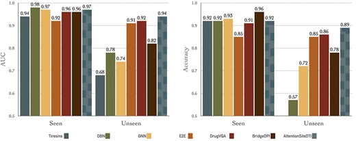
Comparison of AttentionSiteDTI with six baselines: (left) shows Area Under the Curve (AUC) for seen proteins and unseen proteins in the test; (right) shows Accuracy for seen proteins and unseen proteins in the test. Note that the accuracy scores of Tiresias do not show in unseen case because it is lower than the lower bound of the y-axis (0.5). Note that for a head-to-head comparison with all models, including ours, we implemented the BridgeDPI model with our experimental setting. Our model outperforms all other methods in unseen proteins, which means our model is better in generalization than other models. In the seen protein scenario, our model is comparable to other models, and high AUC and accuracy in seen scenario indicate over-fitting of the model.
Discussion
We believe that the improved performance of our proposed model can be explained by several factors, including (1) the input representations, which, as argued in [40], significantly affect the prediction performance of the model. The use of more advanced input feature representations such as structured graphs can help capture the structural information of the molecules, (2) the prediction technique. For example, traditional ML-based techniques such as NNScore and FRscore often depend on the quality of hand-crafted features, which most often fail to learn complex nonlinear relationships in DTI [35]. In contrast, self-attention provides a powerful and automatic feature extraction mechanism to learn higher order nonlinear relationships. Also, deep learning approaches that use string representations as the input to their models are unable to capture the structural information of drugs and/or proteins [41]. On the other hand, graph-based neural networks (that use graph representations of drugs and proteins) can effectively capture topological relationships of drug molecules and target proteins, which enables further performance improvement [41], and most importantly (3) our context-sensitive embedding approach to drug–target complexes. In our approach, a drug–target complex is treated as a sentence with relational meaning between its biochemical entities a.k.a. protein pockets and drug molecule; This enables capturing the most important contextual semantic and relational information in a biochemical sequence (i.e. sentence) for relation classification similar to sentence classification in NLP.
In addition to improved performance, our model enables interpretability by exploring which binding sites of the protein interact with a given ligand. This is especially crucial in the design and development of new pharmaceutically active molecules, where it is critical to know which parts of a molecule are important for its biological properties.
Interpretation Module
Ligands bind to certain parts (active sites) of proteins, either blocking the binding of other ligands or inducing a change in the protein structure, which produces a therapeutic effect. Binding at other sites that provide no therapeutic value is ‘non-active’, and generally does not cause a direct biological effect. Ligands binding to active sites and inducing a change in protein structure (conformation) are less likely in our system of study and are probably not as helpful for building models (usually, these ligands/therapeutic agents are employed/considered when a patient has an ailment, which causes natural biochemicals to be produced in insufficient quantities).
In this work, the attention mechanism enables the model to predict which protein binding sites are more probable to bind with a given ligand. These probabilities are contained in the attention matrix, computed by the model. The attention visualization can be found in Figure 5 as the heat map of the protein for the complex of SARS-CoV2 Spike protein and human, host cell-expressing ACE2 in the interaction with the drug named Darunavir. The projection of the heat map on the protein is depicted in this figure, as well.
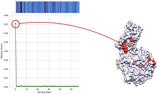
(Left) shows Heatmap and line plot of self-attention mechanism weights for each binding site in the proposed method with the input of Darunavir as ligand and complex of COVID spike protein and ACE2 as protein, which translates to the probability of each calculated binding site of the protein being active for that specific ligand. (Right) shows projected heatmap of self-attention weights on the complex of COVID spike protein and ACE2. This figure shows the interpretability of our model, which can give us the binding site that has the most probability of binding to the ligand.
In-Lab Validation
SARS-CoV-2 Case study
To further evaluate the practical potential of our proposed model, we experimentally tested and validated the binding interactions between spike (or ACE2) protein and seven candidate compounds (N-acetyl-neuraminic acid, 3|$\alpha $|,6|$\alpha $|-Mannopentaose, N-glycolylneuraminic acid, 2-Keto3-deoxyoctonate, N-acetyllactosamine, cytidine5-monophospho-N-acetylneuraminic acid sodium salt and Darunavir). Evaluation was performed using a binding inhibition assay kit. Here, candidate molecules were used as inhibitor compounds toward formation of the spike protein-ACE2 complex. Greater performance, of a given candidate molecule, in these assays translates directly to therapeutic value as formation of this complex has been identified as the first step toward host cell infection by the SARS-CoV2 virus. Interaction between these two proteins is facilitated by a glycans on the host cell. These glycan modifications of surface proteins are unique in composition, surface density and in linkage (i.e. ‘O’ and ‘N’ type); as well as often being cell type and tissue-specific [42]. The glycan modifications on ACE2 are common for cells of the respiratory system (oral cavity, lung epithelial cells), allowing recognition by certain upper respiratory tract infecting viruses (e.g. SARS-CoV2, porcine epidemic diarrhea virus and alphacoronavirus transmissible gastroenteritis virus) [43, 44]. It has been shown that SARS-CoV2 binds specifically to neuraminic acid modifications on the ACE2 host cell surface. Therefore, we have chosen N-acetyl-neuraminic acid as a model/standard inhibitor molecule in our study (i.e. free/soluble N-acetylneuraminic acid can bind the spike protein and preclude complex formation). To assess the sensitivity of our model, our set of candidate molecules was chosen to be reflective of small chemical/structural changes to the standard N-acetylneuraminic acid reference. N-acetylneuraminic acid is also known as sialic acid and marks the simplest composition for a set of similar chemicals grouped as sialic acids. Several of our chosen candidate molecules were chosen from this chemical family. Cytidine5-monophospho-N-acetylneuraminic acid possess a simple nucleotide modification, which has a similar binding character as neuraminic acid (via complementarity) to common binding partner molecules. N-glycolylneuraminic acid is highly similar to N-acetylneuraminic acid in structure and composition, differing only in an oxidation of the acetyl group to a carboxylic. 2-Keto3-deoxyoctonate is a sialic acid which does not possess the nitrogen-acetyl substituent found for N-acetylneuraminic acid: altering the molecules hydrophilicity. In many cases, glycans are formed as oligosaccharides. Therefore, a disaccharide N-acetyllactosamine molecule was included, as well as the polycyclic 3,6-mannopentaose saccharide. Lastly, the potential for generalized identification of therapeutics toward SARS-CoV2 was assessed by inclusion of the small drug molecule darunavir in the evaluation set. As the results show in Table 8, we observe high agreement (five out of seven matched results) between the predicted and experimentally measured DTIs, which illustrates the potential of our AttentionSiteDTI as an effective complementary pre-screening tool to accelerate the exploration, and recommendation of lead compounds with desired interaction properties toward their targets. In our experiment, we set the activity threshold to 15 nM to only capture highly active compounds, thereby limiting the influence of interactions at neighboring sites and weak interactions with poor coordination to the binding site center.
In-lab Validation of AttentionSiteDTI in the case study of Covid-19
| Compound | AttentionSiteDTI | Lab Results |
|---|---|---|
| 2-keto-3-deoxynononic acid | Noninteracting | Interacting |
| N-Glycolylneuraminic acid | Noninteracting | Interacting |
| Cytidine-5-monophospho-N-acetylneuraminic acid sodium salt | Interacting | Interacting |
| Darunavir | Interacting | Interacting |
| N-acetyl-neuraminic acid | Noninteracting | Noninteracting |
| N-Acetyllactosamine | Noninteracting | Noninteracting |
| 3,6-Mannopentaose | Noninteracting | Noninteracting |
Conclusion
In this work, we proposed an end-to-end GCNN-based model, built on a self-attention mechanism, to capture any relationship between binding sites of a given protein and the drug in a sequence analogous to a sentence with relational meaning between its biochemical entities a.k.a. protein pockets and drug molecule. Our proposed framework enables learning which binding sites of a protein interact with a given ligand, thus allowing interpretability and better generalizability, while outperforming state-of-the-art methods in the prediction of DTI. We experimentally validated the predicted binding interactions between seven candidate compounds and the Spike (or ACE2) protein. The results of our in-lab validation showed high agreement between the computationally predicted and experimentally observed binding interactions. Our model exhibits state-of-the-art performance, is highly generalizable, provides interpretable outputs and performs well when validated against in-lab experiments. As a result, we expect it to be an effective virtual screening tool in drug discovery applications.
We proposed a new formulation of DTI prediction problem similar to sentence classification in NLP. In this new formulation, we treated a biochemical sequence (drug–target complex) as a natural language sentence. This enables capturing contextual and relational information contained in the sentence.
A graph-based deep learning model was developed to solve the DTI prediction problem in an end-to-end manner, where both the graph embeddings and the DTI prediction model were learned simultaneously. This enables more efficient and effective training of the network as a whole with minimizing over one loss function.
We proposed using graph representations of both drug and target as the inputs to the network. More specifically, we used graph representations of protein pockets as inputs for the target protein, which helps with better generalizability of the model.
We devised self-attention mechanism that enables interpretability through identification of most probable binding sites of a protein with a given ligand.
Our proposed model showed improved performance compared with many state-of-the-art models in terms of several performance metrics on three benchmark datasets.
We validated the practical potential of our computation model through in-lab validation, where we measured the binding interaction between several compounds and Spike (ACE2) protein, and compared the results with computational predictions.
We observed high agreement between computationally predicted and experimentally observed binding interactions, which illustrates the potential of our model in virtual screening tasks.
Data and Code availability
All datasets are publicly available. DUD-E dataset is available at http://dude.docking.org, Human dataset is available at https://github.com/IBMInterpretableDTIP and finally the customized BindingDB-IBM dataset can be found at https://github.com/masashitsubaki/CPI_prediction/tree/master/. We used 3D structures of proteins in the Human dataset from https://github.com/prokia/drugVQA. Also, all instructions and codes for our experiments are available at https://github.com/yazdanimehdi/AttentionSiteDTI.
Acknowledgments
We thank Ms.Katalina Biondi for discussions and her valuable feedback and comments on earlier versions of the manuscript.
Author Biographies
Mehdi Yazdan-Jahromi is a second year PhD student at University of Central Florida. His current research interests include Graph Neural Networks, Algorithmic Fairness.
Niloofar Yousefi is a Postdoctoral Research Associate at UCF’s Complex Adaptive Systems (CAS) laboratory in the collage of Engineering and Computer Science. Her research areas include Machine Learning, Artificial Intelligence and Statistical Learning Theory to develop data analytics solutions with more transparency and explainability.
Aida Tayebi is a second year PhD student at University of Central Florida. Her current research interests include Algorithmic Fairness, and bias mitigation techniques in DTI.
Ozlem Ozmen Garibay is an Assistant Professor of Industrial Engineering and Management System at the University of Central Florida where she directs the Human-Centered Artificial Intelligence Research Lab (Human-CAIR Lab). Prior to that, she served as the Director of Research Technology. Her areas of research are big data, social media analysis, social cybersecurity, artificial social intelligence, human-machine teams, social and economic networks, network science, STEM education analytics, higher education economic impact and engagement, artificial intelligence, evolutionary computation and complex systems.
Sudipta Seal is currently the chair of the Department of Materials Science and Engineering at University of Central Florida, as well as a Pegasus Professor and a University Distinguished Professor. He joined the Advanced Materials Processing and Analysis Center and UCF in 1997. He has been consistently productive in research, instruction and service to UCF since 1998. He has served as the Nano Initiative coordinator for the vice president of research and commercialization. He served as the director of AMPAC and the NanoScience Technology Center from 2009 to 2017.
Elayaraja Kolanthai is a Postdoctoral Research Associate at UCF’s Materials Science and Engineering. His current research interests include Development of nanoparticles, layer-by-layer antimicrobial/antiviral nanoparticle coating, polymer composites for tissue engineering and gene/drug delivery application.
Craig J. Neal is a Postdoctoral Research Associate at UCF’s Materials Science and Engineering. His current research interests include Wet chemical synthesis and surface engineering of nanoparticles for biomedical applications and electrochemical devices. Electroanalysis of nanomaterials and bio–nano interactions.
References
Author notes
Mehdi Yazdani-Jahromi and Niloofar Yousefi contributed equally.
