miRe2e: a full end-to-end deep model based on transformers for prediction of pre-miRNAs

Abstract

Motivation

MicroRNAs (miRNAs) are small RNA sequences with key roles in the regulation of gene expression at post-transcriptional level in different species. Accurate prediction of novel miRNAs is needed due to their importance in many biological processes and their associations with complicated diseases in humans. Many machine learning approaches were proposed in the last decade for this purpose, but requiring handcrafted features extraction to identify possible de novo miRNAs. More recently, the emergence of deep learning (DL) has allowed the automatic feature extraction, learning relevant representations by themselves. However, the state-of-art deep models require complex pre-processing of the input sequences and prediction of their secondary structure to reach an acceptable performance.

Results

In this work, we present miRe2e, the first full end-to-end DL model for pre-miRNA prediction. This model is based on Transformers, a neural architecture that uses attention mechanisms to infer global dependencies between inputs and outputs. It is capable of receiving the raw genome-wide data as input, without any pre-processing nor feature engineering. After a training stage with known pre-miRNAs, hairpin and non-harpin sequences, it can identify all the pre-miRNA sequences within a genome. The model has been validated through several experimental setups using the human genome, and it was compared with state-of-the-art algorithms obtaining 10 times better performance.

Availability and implementation

Webdemo available at https://sinc.unl.edu.ar/web-demo/miRe2e/ and source code available for download at https://github.com/sinc-lab/miRe2e.

Supplementary information

Supplementary data are available at Bioinformatics online.

1 Introduction

MicroRNAs (miRNAs) can regulate genes, determine the genetic expression of cells, influence the state of the tissues and promote or inhibit certain diseases and infections (Bartel, 2004). The discovery of new miRNAs and their function is necessary for better understanding their roles in genes regulation. The precursors of miRNAs (pre-miRNAs) generated during biogenesis have a well-known RNA secondary structure, which has allowed the development of computational algorithms for their identification. The pre-miRNAs typically exhibit a stem-loop structure, which are also known as hairpin, with few internal loops or asymmetric bulges. However, a very large amount of hairpin-like structures can be found in a genome, thus the discovery of truly pre-miRNAs remains a challenge.

For the prediction of pre-miRNAs, there is a large number of pipelines that use genomics data as input for building a binary classifier based on machine learning (ML) (Bugnon et al., 2021; Stegmayer et al., 2019). All of them need an intensive pre-processing of the raw genome: set a window length, go through the genome and cut it into fixed sequences, calculate the corresponding secondary structure, check that it forms a hairpin and discard those sequences that do not (named flats). Then, a large number of handcrafted features are extracted from the harpins, such as the number of loops or the minimum free energy when folding the secondary structure (MFE), among many others (de Lopes et al., 2014; Raad et al., 2020; Yones et al., 2015). The MFE has proved to be an important feature for distinguishing pre-miRNAs (Bartel, 2004). This feature extraction step is highly dependent on the manual selection of many parameters, and these human decisions in pre-processing can have an impact in the prediction afterward. The ML classifiers are then trained to learn those features from positive (well-known pre-miRNAs deposited in miRBase) and negative class samples, for the discovery of new pre-miRNAs in non-coding and non-repetitive regions of any genome.

In several bioinformatics domains, the big challenge today is the development of ML methods without requiring any pre-processing of the input, that is, a so-called end-to-end model (Chaabane et al., 2019; Trieu et al., 2020; Tsubaki et al., 2018). In the scenario of genome-wide pre-miRNAs prediction, such a method should be able to be trained only with raw RNA sequences (no features), and then be able to receive the raw genome of any species without any features extraction nor calculation of secondary structure, to identify hairpin-like pieces of RNA highly likely to be novel pre-miRNAs. However, since in such a scenario, it is not possible to previously discard those sequences that do not fold as hairpins (the flats), it is necessary to incorporate all them into the training. Precisely for avoiding any feature engineering step, the emergence of deep learning (DL) has produced meaningful improvements in the field of automatic representation for computer vision, speech recognition and many other application domains (LeCun et al., 2015). Deep models can automatically extract relevant features by themselves, directly from raw data, and those are considered today the best paradigm of ML for most classification tasks (Bengio et al., 2013; Jurtz et al., 2017). DL has already been used for small-RNA feature extraction, identification and classification (Amin et al., 2019; Zeng et al., 2016; Zheng et al., 2019). In addition, DL can detect motifs in a set of homologous sequences, which are then the key for distinguishing among different types of protein families or predict its structure (Senior et al., 2020; Seo et al., 2018). In Eraslan et al. (2019), authors analyze gaps and challenges for DL in genomics, mentioning the need for more DL-based tools capable of handling the real genome-wide scenario with full end-to-end models, without requiring any type of handcrafted pre-processing.

In this line of work, very recently a model based on convolutional neural networks (CNN), named deepMir, has been proposed for classification of miRNA families (Tang and Sun, 2019). Differently from most binary classification tools, the focus here is on classifying input sequences into different miRNA families for more detailed function annotation. It receives as input only RNA sequences, using a one-hot-encoding scheme to convert a RNA sequence of $1\times N$ nt into an $4\times N$ matrix to feed the network, coding this way the 4 nucleotides types in the sequence. The CNN model contains two convolutional layers, followed by max pooling layers and three fully connected layers with dropout. The model is trained with pre-miRNAs from Rfam and mature miRNAs from miRBase. In Bugnon et al. (2021), it was shown that the performance of deepMir was below those deep models that use also the predicted secondary structure as input, such as deepMiRGene (Park et al., 2017) and mirDNN (Yones et al., 2021), which receives also the MFE. However, deepMir is an important step toward models fully trainable from raw genomic sequences and a starting point for achieving end-to-end models, with the potential of outperforming other approaches thanks to the capability of learning the features automatically. Nevertheless, it should be noted that deepMir has not been designed nor tested for discovery of novel pre-miRNAs in a genome-wide scenario. Moreover, pure CNNs have shown some limitations for the analysis of sequences, due to the locality of its convolutions and the loss of long-term dependencies, requiring the stacking of several layers (Vaswani et al., 2017).

In the last 5 years, many reviews have experimentally compared ML and DL tools for pre-miRNA prediction, in the same conditions and datasets (Demirci et al., 2017; Stegmayer et al., 2019). In Park et al. (2017) deepMirGene was compared against the best ML methods, showing that the DL model performance was superior. In Stegmayer et al. (2019), ML tools based on Random Forest, Naive Bayes, Support Vector Machines and DL-based methods were evaluated for several class imbalances, under conditions similar to those found in a real genome-wide prediction. In that work, the performance of methods based on classical ML was overcome by DL-based methods in high imbalance situations. More recently, in Bugnon et al. (2021), a comparison of the different DL methods proposed to date (deepMir, deepMirGene, deepBM, deeSOM, etc.) was made in genome-wide conditions with high class imbalance. It was found that deepMirGene obtained the best performance using sequence and structure as input, and deepMir using only sequence obtained a close good performance. Both methods outperformed the other models in the prediction of pre-miRNAs in the human genome. More recently, mirDNN has appeared as the best predictor for genome-wide. Based on all these previous experiments, it can be stated that these methods are the more challenging and best-performing DL models for pre-miRNAs prediction up to date.

As an alternative to improve DL models in the automatic extraction of features, the Transformers have appeared very recently, coming from the natural language processing domain (Devlin et al., 2018; Vaswani et al., 2017). Transformers are deep networks with self-attention mechanisms in each layer, which allows obtaining several improvements with respect to recurrent and CNN models (Dosovitskiy et al., 2020). In the past 2 years, Transformers have also arrived to the modeling macromolecules including proteins (Clauwaert et al., 2021; Rives et al., 2021), DNA (Ji et al., 2020; Le et al., 2021; Nambiar et al., 2020; Rao et al., 2021) and RNA (Wan et al., 2019). The information flow in Transformers is parallelized, instead of being done sequentially as in recurrent networks. Moreover, unlike convolutional networks that work with a local vision and require many layers to obtain a global vision, the attention mechanisms allow the analysis of longer sequences without losing context information, thus maintaining a global vision of the input in each layer, due to their point-to-point connections (Vaswani et al., 2017). These characteristics of the Transformers can allow learning relationships between all nucleotides within a sequence, thus being able to better model its secondary structure. This way, it is possible to develop a DL model capable of, only from the raw RNA sequence, extracting information about its secondary structure without any data pre-processing nor engineered feature extraction. Being precisely the secondary structure one of the most important characteristics for the pre-miRNA classification (de Lopes et al., 2014), most DL models propose to use a 2D mapping of the RNA sequence, then applying 2D CNN to process this matrix and obtain a contact point matrix of size L × L, which requires considerable processing without significantly increasing the accuracy of the prediction (Singh et al., 2019). To better solve these issues we propose a Transformers-based architecture, where thanks to the point-to-point product of its attention mechanisms it is possible to efficiently replace the 2D mapping. As an additional advantage, instead of obtaining a contact matrix at the output, a model based on Transformers can directly provide the secondary structure, with the classical format of parentheses and points in a single row. Furthermore, once trained, Transformers can significantly speed up the estimation of structures and the final pre-miRNA prediction.

In this work, we propose miRe2e, a full end-to-end DL model for pre-miRNA prediction based on Transformers and attention mechanisms. It is capable of receiving as input the sequences of raw genome-wide data, without any pre-processing. After a training step with known and unlabeled sequences, it can identify pre-miRNA sequences within a genome. This model automatically learns the intrinsic structural characteristics of precursors of miRNAs from the raw data, without any feature engineering. The proposal has been tested with several experimental setups with the human genome, and compared with state-of-the-art algorithms.

2 Full end-to-end DL model

The miRe2e is a full end-to-end DL model based on Transformers. A Transformer is a neural model architecture that relies on attention mechanisms to infer global dependencies between input and output. Each Transformer is made up of layers of attention mechanisms and feedforward networks (Vaswani et al., 2017). The attention mechanisms aim at finding relationships between each pair of elements within a sequence (i.e. between nucleotides in a genomic sequence) (Bahdanau et al., 2015). To do this, a dot product is calculated between each pair of elements, thus obtaining a score matrix. Then, softmax is applied to each row of the matrix, obtaining the weights associated with the product of each nucleotide with the rest of the nucleotides in the sequence. For obtaining the new vector associated with each nucleotide, a dot product is made between its weight vector, that is the corresponding row of the score matrix, and the full sequence. Finally, an output sequence of the same dimension as the input sequence is obtained, but where each nucleotide is weighted by its importance in its context. In particular, several sets of these weights can be learnt to capture different relationships in the sequence, giving rise to the so-called multi-head attention (Vaswani et al., 2017). In this case, instead of using a single large weights matrix, each nucleotide is projected in parallel into a set of matrices of less dimension, which are called heads. The output of each head is concatenated into a single vector, which is projected to obtain a single output. This allows the model to obtain information from different subspaces, thus achieving a better representation for each nucleotide position in the sequence.

The aim of miRe2e is to analyze a raw genome-wide sequence in the search for pre-miRNA candidates. To do so, shorter sequences are obtained with a sliding window of length L and step s. The model receives each one of these sequences and gives a pre-miRNA score. Thus, after the training stage, the model can run over any genome-wide sequence and indicate the positions where there might be a possible pre-miRNA. Each of the windowed sequences is embedded in a $L\times 4$ one-hot-encoding tensor, where each column represents one of the four possible nucleotides (A, C, G, U) at each position. The miRe2e processes this input with three internal deep models, as depicted in Figure  1: the Structure Prediction (A), the MFE Estimation (B) and the pre-miRNA Classifier (C). The figure shows the complete miRe2e model, where the input/outputs of each model are shown with numbers and the details of the neural architecture of each model are shown immediately below. The Structure Prediction model allows obtaining the secondary structure from an RNA input sequence. The MFE Estimation model calculates the MFE from an input RNA sequence and its corresponding secondary structure. Finally, the last deep model performs the pre-miRNA classification.

Fig. 1.

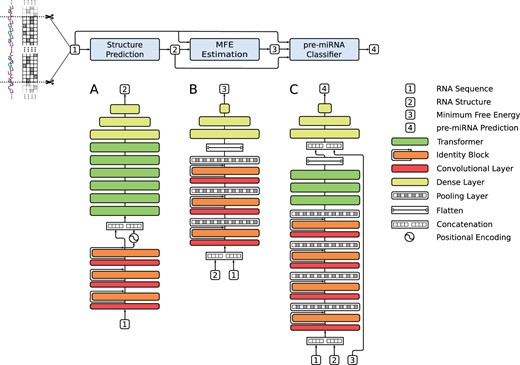
Schematic representation of the complete miRe2e: full end-to-end architecture for pre-miRNA prediction in genome-wide data. The details of the architecture of each model are shown below. (A) The input RNA sequence enters the Structure Prediction model, which outputs the RNA structure . (B) The MFE Estimation model receives and and calculates the Minimum Free Energy . (C) The pre-miRNA Classifier model receives , and and provides the pre-miRNA prediction

The Structure Prediction model (Fig.  1A) learns to estimate the secondary structure from an RNA sequence. Here the one-hot-encoding tensor 1 enters a CNN of three stages, each one with identity blocks. Each one of these identity blocks is made up of two activation functions, two batch normalization layers, two 1D convolutional layers of length L, and w_A filters with identity shortcut connections (He et al., 2016). The main function of this part of the model is to automatically extract motifs from the input sequence and increase the number of features to allow a fast processing in attention layers (Vaswani et al., 2017). At the output of the CNN, the positional encoding signal is added to each embedding (Vaswani et al., 2017). Then, there is a stack of six Transformer encoders. In this part of the model, each encoder layer is composed of w_A input features, h_A heads and n_A neurons in the hidden layers of each feedforward network, where the number of hidden neurons is set to $n_A=4w_A$ as suggested in Vaswani et al. (2017). The function of this encoder is, through its attention mechanisms, to model the contact matrix of each nucleotide in the input sequence, thus being able to estimate its secondary structure. Finally, after the encoder there is a 3-layer multilayer perceptron (MLP), ELU activation functions in the hidden layers and hyperbolic tangent functions at the output are used. Since in Transformer encoders the output has the same dimension as the input (⁠$L\times w_A$⁠), and the MLP is applied to each sample of the input tensor without flattening, a reduction in the dimension of features from w_A to 1 is obtained, generating a tensor of $L\times 1$ at the output 2. To avoid the bias toward the non-pre-miRNA sequences due to the high class-imbalance, class oversampling was done, where each training batch is constructed with the same number of samples from the minority class (actual pre-miRNAs) and the majority class. To do this, the minority class was sampled with replacement. Finally for this model, the mean squared error (MSE) loss function was used for training, which is calculated between the estimated $L\times 1$ output tensor and the reference secondary structure. This was represented with 0, 1 and -1 for unmatched nucleotides, matches in the 5′ strand and matches in the 3′ strand, respectively. Thus, it is possible to encode the two strands of each hairpin into a single real vector.

The second model (Fig.  1B) aims to estimate the MFE from the input sequence and its secondary structure. It receives 1 and 2, concatenates them and obtaining a $5\times L$ tensor with the fifth row being the secondary structure predicted for the input sequence. The model is made up of a 3-stage CNN, each one composed of an identity block and a stacked pooling layer. Due to each pooling layer, after each stage the length of the input tensor is reduced by a factor of 2. At each identity block, the 1D convolutional layers are formed by w_B filters and a $L/(2^N)$ length, where N is the stage number. Then, after a flatten layer, there is a 3-layer MLP where each of these layers has batch normalization and ELU activation functions. MSE loss was used for training, as the error function between each predicted output value and its reference MFE value. The output of this CNN is the estimated MFE 3 of the sequence.

The pre-miRNA Classifier model (Fig.  1C) classifies the input sequence 1, with its secondary structure 2 and the estimated MFE 3. This model has a 4-stage CNN, each made up of three identity blocks with w_C filters and a stacked pooling layer. Then, there is a stack of three Transformers encoders. Each encoder layer has w_C input features, h_C heads and n_C neurons in the hidden layers of each feedforward network. Its function is to encode the sequential information of the input, thus modeling the dependency between each nucleotide in a global way. After the encoder, the $w_C\times L/16$ output tensor is flattened and concatenated with the output of the MFE model 3. After that, it goes to a 4-layer MLP, hidden ELU activation functions, batch normalization and dropout. Finally, a softmax layer at the output predicts the corresponding class for the input sequence 4. Since miRe2e is composed of three models in cascade, a 3-stage training was carried out, where the output of each model was the input of the next one. More details about the miRe2e hyperparameters and training can be found in the Supplementary Material.

3 Materials and methods

3.1 Data

Genome-wide data of Homo sapiens (http://ftp.ensembl.org/) was used in all the experiments (Bugnon et al., 2019). For training the first model (secondary structure prediction), all the metazoan pre-miRNAs (23 178), excluding H.sapiens, obtained from mirBase v.22 (http://www.mirbase.org/) were used, and 2 000 000 pseudo-hairpins were extracted from the genome with HextractoR (Yones et al., 2020). For the secondary structure used as reference to train the structure prediction model, two models were evaluated: the well-known RNAfold (Hofacker, 2003) and a recent model based on DL called Spot-RNA (Singh et al., 2019). A better performance was found when miRe2e was trained with the structures generated by RNAfold. We believe this might be due to the fact that Spot-RNA was not trained specifically with pre-miRNA structures, and could be biased toward other types of RNA structures. Thus, to train miRe2e, the target structure to be predicted for each input sequence was its corresponding secondary structure predicted with RNAfold, at a temperature of 37°C. Regarding diversity of the pre-miRNAs in the dataset, it should be mentioned that in spite the miRNA families contain similar entries, families are defined according to the seed of the mature miRNA (Bartel, 2018) and not taking into account the complete pre-miRNA structure, which is the input of miRe2e.

For training the deep model that estimates the MFE, the secondary structure predicted by the first model and its respective input RNA sequence are required. The desired output here was the RNAfold predicted MFE value normalized by sequence length. For this model, 23 178 metazoan pre-miRNAs (excluding H.sapiens) were used. In addition, 48 000 pseudo-hairpins obtained with HextractoR and 48 000 sequences that did not form hairpins (flats) were randomly extracted from the genome. For testing the complete model, the input sequences are obtained through a scan and cut of each chromosome with overlapped windows (length 100 nt, step 20 nt).

3.2 Performance evaluation

The methods performance is reported with standard recall or sensitivity (s⁺), precision (p) and F₁ evaluation metrics,

$$s^{+}=\frac{TP}{TP+FN},\hspace{0.17em}\hspace{0.17em}\hspace{0.17em}\hspace{0.17em}p=\frac{TP}{TP+FP},\hspace{0.17em}\hspace{0.17em}\hspace{0.17em}\hspace{0.17em}{F}_1=2\hspace{0.17em}\frac{s^{+}\hspace{0.17em}p}{s^{+}+p},$$

where TP, FP and FN are the number of true positives, false positives and false negatives, respectively. The recall measures how good a classification method is for recognizing the TPs of the task. The precision measures the relation between TPs and FPs. In a realistic scenario for practical applications, precision is very important for datasets with high class imbalance, because FPs can be many more than the TPs. Thus, considering the characteristics of the classification task under study, it is important to take into account both sensitivity and precision. Therefore, F₁ is used as a global comparative measure.

It should be noted here that in this scenario of such high-class imbalance, very low values can be expected from these measures. For example, if a predictor has only 1% of FP in a dataset with 1,000 TP and 10,000,000 total sequences, the precision could be below 0.001. As a consequence, very low values of F₁ will be also observed. For performance evaluation and comparison with other methods, a 4-fold stratified cross-validation strategy was used, that is, preserving the original percentage of each class on each fold.

These measures were also used to obtain precision–recall curves (PRC), which is a well-known indicator for global performance of classifiers. It has been shown (Saito et al., 2015) that this measure is preferred over the classical receiver operating characteristic (ROC) curve to assess binary classifiers on highly imbalanced data. When there is a large class imbalance in a dataset, a classifier can reach a good performance in terms of specificity (and sensitivity), but can perform poorly in providing good quality candidates, with a large amount of false positives. A PRC can provide a better assessment of performance because it also evaluates the fraction of true positives among the total positive predictions. The area under the precision–recall curve (AUCPR), which is a single numeric summary of the information, will also be reported as a global measure along all the possible output thresholds in the compared models.

4 Results

4.1 Generalization capability on cross-validation setup

To show the generalization capability of our model, a comparison of predictions in cross-validation for the chromosome 1 of H.sapiens was done. This chromosome was selected because it is the one with the largest number of positive cases, which is important to reduce the results variance in a cross-validation setup (full results for each chromosome will be presented in Section 4.3). Training data included all positives (156 known pre-miRNAs) in chromosome 1 and the rest of the sequences of chromosome 1 (more than 24 000 000), divided into 4-folds for training and testing. We compared the performance obtained with miRe2e for this task against the most recently proposed pre-miRNA prediction tool, deepMir (Tang and Sun, 2019), which also receives raw input sequences (i.e. without preprocessing and feature extraction). In this setup, deepMir was re-trained with the same training sets that our model, changing the output layer for binary prediction with a softmax activation function.

The results are shown in Table  1, which reports each fold results in the rows, and then s⁺, p and F₁ for each method, respectively. Regarding s⁺, both methods have good results, being deepMir slightly better on average. Instead, the precision of miRe2e is always the best one, in all folds. It is quite remarkable here that the performance of miRe2e is one order of magnitude higher than deepMir. This is precisely reflected by F₁, where miRe2e is always superior to deepMir, in all cases with one order of magnitude of difference. This is due to the fact that miRe2e can effectively model the secondary structure of the RNA sequence, and since this information is key for filtering false positives. The model can improve p without a drop in s⁺, thus increasing the global F₁. It should be noted that these significant results were obtained in the context of the high-class imbalance of one chromosome (156 positive versus 24 000 000 negative samples), which suggest that the performance of miRe2e in a complete genome-wide scenario can be superior to deepMir.

Table 1.

Performance comparison of miRe2e and deepMir for the prediction of pre-miRNAs in the chromosome 1 of H. sapiens. Bold indicates best performance

Fold	s+		p		F1
	miRe2e	deepMir	miRe2e	deepMir	miRe2e	deepMir
1	0.0130	0.0250	0.0020	0.0002	0.0030	0.0005
2	0.0130	0.0130	0.0020	0.0004	0.0040	0.0008
3	0.0380	0.0130	0.0010	0.0006	0.0020	0.0012
4	0.0130	0.1150	0.0110	0.0005	0.0120	0.0011
Avg.	0.0193	0.0415	0.0040	0.0004	0.0052	0.0009

4.2 Prediction of human pre-miRNAs added in the future in miRBase

To further test the performance of miRe2e in a more realistic scenario, involving the prediction of novel pre-miRNAs in the future, we trained it on the human pre-miRNAs dataset from miRBase v21 (2014) and tested with the human pre-miRNAs introduced afterwards in miRBase v22 (2018). The training set has 1854 positive, 87 500 negative and 787 500 flat sequences and the test set was composed of 27 positive, 12 500 negative and 112 500 flat sequences. We have verified that pre-miRNAs from v21 then removed in v22 were not used for training. In addition, we checked for miRTrons in the training and testing sets, due to their difference in trinucleotide content with respect to miRNAs (Zhong et al., 2019). We found that the training set has 234 miRTrons, and there are only 2 new miRTrons in the testing set, which were correctly predicted by our model.

The PR curves are shown in Figure  2 for both models in different colors. It can be seen that miRe2e (blue line) has reached the best results, with AUCPR $=0.17$⁠. The deepMir method (orange line) has obtained AUCPR $=0.08$⁠, a very low value and half than that of miRe2e. It should be noticed that, for the same recall in both methods (e.g. 0.20), while miRe2e obtains a $F_1=0.26$ with 11 FP, deepMir has $F_1=0.08$ with 113 FP (more than 10 times). This is of high importance in the application domain, where if for the same TP rate a large number of initial candidates to novel pre-miRNAs are obtained, in the order of hundreds or thousands, it will be almost impossible to validate them all experimentally to discover real pre-miRNAs. Thus, a smaller number of predicted and good candidates is preferred. In addition, in a detailed analysis of the negative training set we have found a few entries that were subsequently added as novel pre-miRNAs to miRBase. From the 27 positive samples in the test set, 26 were correctly predicted by our model. This shows that the performance of the classifier was not affected by some mislabeled cases in the training set. These results show that miRe2e is effective for the prediction and discovery of new pre-miRNAs in the future.

Fig. 2.

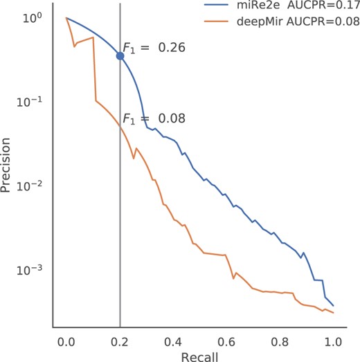
Precision recall curves for miRe2e and deepMir, for the prediction of human pre-miRNAs recently added in miRBase

4.3 Genome-wide discovery of pre-miRNAs in a new species

Finally, to test miRe2e in a very realistic task of discovery novel pre-miRNAs in a new species, the following experimental setup has been used. The Structure Prediction model was trained with all known metazoan pre-miRNAs excluding H.sapiens (23 048 sequences), and negative samples from animals (2 000 000 hairpins in total from Anopheles gambiae, Drosophila melanogaster and Caenorhabditis elegans) (Bugnon et al., 2019). The MFE model was trained with all known metazoan pre-miRNAs excluding H.sapiens, 48 000 pseudo-hairpins and 48 000 flats randomly extracted from Anopheles gambiae, Drosophila melanogaster and Caenorhabditis elegans. The pre-miRNA Classifier model was trained with all known metazoan pre-miRNAs excluding H.sapiens (23 048), and negative samples from animals (1 000 000 in total from Anopheles gambiae, Drosophila melanogaster and Caenorhabditis elegans: 100 000 hairpins and 900 000 flats). The task was the discovery of all the pre-miRNAs in the human genome (as if it were a novel species recently discovered). Thus, for testing, all the sequences within each chromosome containing a known pre-miRNA, according to the positions described in miRBase v22, were used as the positive class, and the negatives were all the corresponding sequences from the rest of the chromosome.

The results are presented in Table  2. The first column indicates the chromosome, and the second and third column the number of positive and negative examples in that chromosome, respectively. Then the performance of each method is reported with s⁺, p, F₁, AUROC and AUCPR. Finally, the last row indicates the final performance measured in the full human genome. It should be noticed the very large class imbalance that exists in each chromosome. For example, in chromosome 1 there are 156 positives and more than 24 millions of negatives, that is, an imbalance ratio of about 1:160 000. Even worst, in chromosome Y, there are only 4 positives and more than 5 millions of negatives, making the imbalance ratio up to 1:1 430 000. As stated in Section 3.2, in such scenarios, very low values of F₁ can be expected. Note that in this case, with just 1% of FP, the F₁ drops below 0.0001, thus the global measures of AUROC and AUCPR are an important complement for the analysis of these results.

Table 2.

Performance comparison of miRe2e and deepMir for the prediction of pre-miRNAs in the genome of H.sapiens

Chr	Pos	Negatives	deepMir					miRe2e
			s+	p	F1	AUROC	AUCPR	s+	p	F1	AUROC	AUCPR
1	156	24 895 488	0.013	0.0020	0.0035	0.7115	0.00004	0.235	0.0040	0.0079	0.9439	0.11880
2	116	24 213 504	0.075	0.0002	0.0003	0.7081	0.00003	0.271	0.0038	0.0075	0.9640	0.13673
3	96	19 826 688	0.063	0.0001	0.0002	0.7024	0.00002	0.240	0.0043	0.0085	0.9623	0.12117
4	62	19 015 680	0.172	0.0000	0.0001	0.7442	0.00002	0.190	0.0025	0.0050	0.9724	0.09576
5	76	18 149 376	0.013	1.0000	0.0263	0.6978	0.01335	0.280	0.0045	0.0089	0.9585	0.14131
6	71	17 080 320	0.071	0.0001	0.0002	0.7885	0.00002	0.271	0.0043	0.0084	0.9771	0.13684
7	82	15 931 392	0.013	0.0004	0.0008	0.7880	0.00004	0.138	0.0019	0.0038	0.9537	0.06949
8	90	14 512 128	0.012	0.0030	0.0048	0.7488	0.00016	0.232	0.0044	0.0086	0.9196	0.11732
9	88	13 836 288	0.012	0.0014	0.0025	0.6767	0.00003	0.318	0.0056	0.0109	0.9580	0.16041
10	69	13 375 488	0.030	0.0001	0.0003	0.7041	0.00003	0.333	0.0044	0.0086	0.9676	0.16804
11	102	13 504 512	0.040	0.0004	0.0007	0.8100	0.00008	0.228	0.0042	0.0082	0.9669	0.11528
12	80	13 326 336	0.013	0.0526	0.0206	0.7694	0.01288	0.231	0.0042	0.0082	0.9382	0.11621
13	40	11 433 984	0.025	0.0000	0.0001	0.7227	0.00001	0.150	0.0027	0.0053	0.9581	0.07596
14	99	10 702 848	0.041	0.0004	0.0009	0.7364	0.00004	0.204	0.0061	0.0119	0.9726	0.10385
15	71	10 199 040	0.044	0.0002	0.0005	0.6519	0.00003	0.324	0.0066	0.0129	0.9564	0.16360
16	82	9 031 680	0.148	0.0003	0.0007	0.6709	0.00009	0.210	0.0035	0.0069	0.9427	0.10615
17	110	8 325 120	0.075	0.0002	0.0004	0.6709	0.00004	0.142	0.0028	0.0054	0.9501	0.07162
18	35	8 036 352	0.031	0.0001	0.0003	0.6778	0.00002	0.250	0.0040	0.0080	0.9430	0.12595
19	143	5 861 376	0.007	0.0014	0.0024	0.8321	0.00018	0.300	0.0077	0.0150	0.9661	0.15277
20	48	6 438 912	0.021	0.0024	0.0043	0.7646	0.02131	0.234	0.0034	0.0067	0.9727	0.11774
21	33	4 669 440	0.032	0.0067	0.0111	0.7025	0.03229	0.161	0.0034	0.0067	0.9610	0.08132
22	46	5 861 376	0.068	0.0002	0.0003	0.6272	0.00002	0.295	0.0038	0.0075	0.9412	0.14882
X	118	15 599 616	0.009	0.0013	0.0023	0.7605	0.00003	0.301	0.0096	0.0186	0.9741	0.15368
Y	4	5 720 064	0.250	0.0001	0.0003	0.5668	0.00002	0.500	0.0003	0.0006	0.7954	0.00010
Full	1917	309 547 008	0.004	0.0003	0.0006	0.7117	0.00003	0.244	0.0043	0.0085	0.9595	0.12313

Note: Detailed measures for each chromosome (Chr) and the full genome (Full row).

The results shown in Table  2 indicate that, in spite of the very large class imbalance existing in each chromosome, the miRe2e model has the best results in all cases. With respect to s⁺, miRe2e is twice better than deepMir for all chromosomes. Regarding p, the precision is the best one, even one order of magnitude higher in most cases. In particular, for chromosome 2, the miRe2e performance in precision is 20 times better than deepMir. In the only case where deepMir has p = 1.00 (chromosome 5), it should be noticed however that the corresponding sensitivity is $s^{+}=0.013$ (in contrast to $s^{+}=0.280$ for miRe2e). Although at this $(s^{+},p)$ point deepMir maximizes F₁, this is achieved at the cost of a very low sensitivity. For F₁ and AUROC measures, again, miRe2e clearly outperforms deepMir in all chromosomes. Finally, regarding the best performance measure for this type of problems with very large class imbalance, AUCPR, the best result for each chromosome is indicated in bold. As it can easily be seen from the table, all best results correspond to miRe2e.

As a deeper insight into the model training, we have compared the previous setup where miRe2e was trained with known animal pre-miRNAs, with miRe2e trained with human pre-miRNAs only. In this comparison, a leave-one-chromosome-out was used, which means that miRe2e was trained with all the pre-miRNAs except those of the testing chromosome. The overall performance of the model trained with only human pre-miRNAs was AUCPR = 1e-5, while the model trained with animal pre-miRNAs achieved AUCPR = 0.12313 (last row in Table  2). The difference in these results might be due to the fact that when the model was trained with all animal pre-miRNAs, there were much more positive training samples to learn from, which improved the capability of modelling the positive class, which is especially important in this high-class imbalance scenario.

As a final comparison, not only with DL methods that use raw data but also with one of the best current methods that uses the predicted secondary structure of the sequences, we have made a full genome-wide experiment. Figure  3 shows the PR curves for the complete human genome (using all sequences from all chromosomes), for miRe2e (raw data), deepMir (raw data), deepMiRGene (raw data + secondary structure) and mirDNN (raw data + secondary structure + MFE). Although the last ones are not a full end-to-end deep model because they use the secondary structure predicted by an external non-neural model (RNAfold), they provide a valid comparison with state-of-the-art references. In the top left of Figure  3 it can be clearly seen that the best performance is for miRe2e, with the largest difference with respect to all other methods. At the highest recalls (>0.6), miRe2e behaves equally to deepMiRGene, very close to mirDNN and much better than deepMir. However, note that this part of the PR curve is of very limited practical utility, given the high number of false positives in this highly imbalanced scenario. It should be mentioned that this high performance for miRe2e is obtained without requiring any other information than the raw sequence. Remarkably, in this experiment, the total AUCPR for miRe2e is 0.12313, which is more than 10 times higher than the other methods. Therefore, the maximum F₁ along the PR curve is achieved by miRe2e (F₁ = 0.0085), closely followed by mirDNN (F₁ = 0.0072) and deepMiRGene (F₁ = 0.0069). The worst method here was deepMir, with maximum F₁ = 0.0006.

Fig. 3.

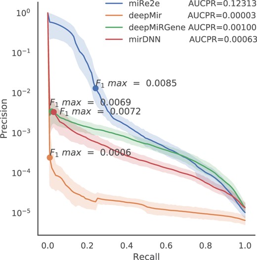
Precision recall curves for miRe2e, deepMir, deepMiRGene and mirDNN for the prediction of human pre-miRNAs in the complete genome

At this point, it was interesting to analyze what contribution each part of the model makes to the final performance of miRe2e. To this end, an ablation study was carried out with chromosome 19, since it is the one with the highest number of positive samples in relation to the negative ones within the human genome (Table  2). The full miRe2e reaches a maximum F₁ = 0.0150. The first part of the ablation study involved removing the MFE prediction model, leaving only the structure + pre-miRNA classification prediction models. In this case, a maximum F₁ = 0.0082 was obtained, that is, a drop of 46%. Then, in a second instance, the MFE and the structure prediction model were both removed, leaving only the sequence as input to the classifier. In this case, the maximum F₁ dropped to 0.0009, which represents a 94% less with respect to the full miRe2e. It can be concluded that each module in miRe2e has a fundamental contribution to the final result, the structure prediction block being the most important one.

These results indicate that miRe2e can be reliably used for the discovery of novel pre-miRNAs in a full genome, with the best possible sensitivity and precision in such a high imbalance scenario. That is, with a very low number of positive examples to learn for the discovery of new ones. This makes miRe2e the first full end-to-end DL model, based in Transformers, for the pre-miRNA prediction task.

5 Conclusions

In this work, we have proposed miRe2e, the first full end-to-end DL model for pre-miRNA prediction in genome-wide data. The advantages of this model over state-of-the methods are twofold. On the one hand, it is capable of receiving raw genome-wide data, without any pre-processing or secondary structure prediction. Thus, it is possible to minimize the impact of handcrafted processes and improve the reproducibility and replicability of results. On the other hand, miRe2e can identify all the pre-miRNA sequences within a genome with very high precision and recall. Moreover, it has shown not to be affected by the very high-class imbalance that exists within a full genome between possible novel pre-miRNAs and the huge amount of negative sequences. In experiments with the human genome, it was able to effectively discover novel pre-miRNAs, even in a future time lapse.

Funding

This work was supported by ANPCyT [PICT 2018 #3384 and PICT 2018 #2905]; and UNL [CAI+D 2016 #082 and CAID 2020 #115]. The authors acknowledged the support of NVIDIA Corporation for the donation of Titan V GPU used for this research.

Conflict of Interest: none declared.