BioProfiling.jl: profiling biological perturbations with high-content imaging in single cells and heterogeneous populations

Abstract

Motivation

High-content imaging screens provide a cost-effective and scalable way to assess cell states across diverse experimental conditions. The analysis of the acquired microscopy images involves assembling and curating raw cellular measurements into morphological profiles suitable for testing biological hypotheses. Despite being a critical step, general-purpose and adaptable tools for morphological profiling are lacking and no solution is available for the high-performance Julia programming language.

Results

Here, we introduce BioProfiling.jl, an efficient end-to-end solution for compiling and filtering informative morphological profiles in Julia. The package contains all the necessary data structures to curate morphological measurements and helper functions to transform, normalize and visualize profiles. Robust statistical distances and permutation tests enable quantification of the significance of the observed changes despite the high fraction of outliers inherent to high-content screens. This package also simplifies visual artifact diagnostics, thus streamlining a bottleneck of morphological analyses. We showcase the features of the package by analyzing a chemical imaging screen, in which the morphological profiles prove to be informative about the compounds' mechanisms of action and can be conveniently integrated with the network localization of molecular targets.

Availability and implementation

The Julia package is available on GitHub: https://github.com/menchelab/BioProfiling.jl. We also provide Jupyter notebooks reproducing our analyses: https://github.com/menchelab/BioProfilingNotebooks. The data underlying this article are available from FigShare, at https://doi.org/10.6084/m9.figshare.14784678.v2.

Supplementary information

Supplementary data are available at Bioinformatics online.

1 Introduction

High-Content Screening (HCS) enables profiling cellular phenotypes across hundreds of thousands of conditions by combining automated microscopy with advanced image analysis methods. HCS thus represents a flexible and cost-effective solution for replacing multiple specific assays (Chandrasekaran et al., 2020; Simm et al., 2018; Way et al., 2021a), and has been widely adopted in both basic and applied research. Notable achievements range from drug discovery (Chandrasekaran et al., 2020; Scheeder et al., 2018; Simm et al., 2018) to the elucidation of combinatorial drug effects (Caldera et al., 2019) and to ex-vivo drug–response screening in patients (Snijder et al., 2017). Depending on the application, the analysis of HCS experiments may involve a variety of tasks. For instance, one might perform a classification task to infer the mechanism of action of candidate drugs (Ando et al., 2017; Ljosa et al., 2013; Pawlowski et al., 2016), compare cellular phenotypes in various conditions (German et al., 2021; Gustafsdottir et al., 2013; Rohban et al., 2017) or describe interactions between cellular perturbations (Billmann et al., 2016; Breinig et al., 2015; Caldera et al., 2019; Fischer et al., 2015; Heigwer et al., 2018). All these cases involve numerous experimental and analytical steps.

A typical HCS experiment starts from preparing microplates with cells subjected to various perturbations, such as different drugs, and stained using standardized protocols, such as the Cell Painting assay (Bray et al., 2016; Fig.  1a). These microplates are then imaged using automated confocal fluorescence microscopy, resulting in a large number of images. Each image is then analyzed to extract quantitative morphological measurements that describe the respective cellular phenotype. Some tools are commonly used for this numerical feature extraction step (McQuin et al., 2018; Pau et al., 2010), and recent deep learning approaches attempt to replace expert-curated measurements with data-driven discriminative features (Ando et al., 2017; Lu et al., 2019; Pawlowski et al., 2016).

Fig. 1.

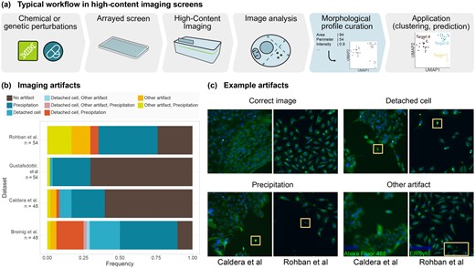
HCS experiments require adequate analysis tools. (a) Standard analysis workflow of HCS experiments. (b) Quantification of imaging artifacts that may lead to biases in HCS analyses in sample images from four published studies (Breinig et al., 2015; Caldera et al., 2019; Gustafsdottir et al., 2013; Rohban et al., 2017). (c) Examples of such imaging artifacts. Boxes highlight regions of interest

While the analytical tasks of HCS experiments vary between applications, they involve common data normalization and filtering steps, and guidelines have been proposed for computing informative representations of cellular phenotypes, usually referred to as morphological profiles (Bougen-Zhukov et al., 2017; Caicedo et al., 2017). An analysis pipeline suitable to facilitate morphological profiling should meet several criteria. First, it should be versatile, to adapt to different HCS use cases and to cope with the diverse challenges inherent to such experiments (Boutros et al., 2015; Caicedo et al., 2017; Chandrasekaran et al., 2020; Ljosa et al., 2013). These challenges include technical problems such as blurred images, poorly adherent cells, saturated pixels, staining artifacts and segmentation mistakes. HCS studies need to address these frequent limitations, as in some experiments most images are affected (Fig.  1b and c). Second, the approach should account for background noise, intensity bias and potential confounders, including plate layout and batch effects. Third, the considerable heterogeneity of the morphological descriptors needs to be handled. Cellular morphology might vary greatly in the analyzed cell populations due to the experimental setup, heterogeneous cell types or cell states, inconsistencies in perturbation efficiency, or when timing-dependent phenomena are imaged as snapshots.

The few actively maintained HCS analysis tools attempting to fulfill these needs include CellProfiler Analyst and its graphical user interface, designed to handle CellProfiler measurements (Jones et al., 2008; McQuin et al., 2018), as well as the general-purpose cytominer and Pycytominer in the R and Python languages, respectively (Becker et al., 2021; Way et al., 2021b). There are also packages addressing similar challenges but focusing on other modalities (which generally provide less spatial information or less throughput than high-content imaging screens) such as the R packages cellHTS2, optimized for measurements from plate readers (Boutros et al., 2006), and more recently cytomapper for analyzing imaging mass cytometry experiments (Eling et al., 2021). Despite the existence of these tools, HCS analysts still heavily rely on custom implementations of morphological profile curation for each study to account for different imaging modalities and analytical goals (Ziegler et al., 2021).

Julia is a high-performance, high-level open-source programming language specifically designed for scientific computing and data science (Bezanson et al., 2017). It is increasingly adopted by researchers in bioinformatics and biomedical research (Roesch et al., 2021), with applications ranging from protein sequence analysis (Zea et al., 2016) to structural bioinformatics (Greener et al., 2020) and flux balance analysis (Heirendt et al., 2017). Julia is also ideal for tackling the challenges of morphological analyses, as they are both computationally demanding and inherently high-level. In this article, we introduce BioProfiling.jl, the first Julia library for efficient and convenient morphological profiling that (i) handles noisy data through systematic filtering and robust statistics, (ii) provides dedicated functions to normalize data and mitigate layout effects and (iii) implements statistical tests for quantifying the strength of morphological changes that take the variability of morphological profiles into account. Our integrated software solution is thus bridging the existing gap between experimental data and biological interpretation. Furthermore, we conduct an image-based chemical screen to validate our approach and characterize the morphological impact of compounds in U-2-OS cells.

2 Materials and methods

2.1 Package implementation and features

We created BioProfiling.jl, a package for the Julia programming language that compiles over 30 methods and data structures for all steps in assembling and curating morphological profiles. To enable the bioimage analysis community to apply BioProfiling.jl to their own data, a complete documentation and a set of notebooks reproducing the analyses described in this paper are provided. In brief, the whole process of morphological profiling is conceptually simplified by defining an Experiment object that includes both quantitative data and metadata in a tabular format, and methods able to interact with these objects directly to curate, transform and visualize the corresponding profiles. After creating the Experiment object from a table of morphological features, such as measurements obtained from CellProfiler (McQuin et al., 2018) or activation values from a deep neural network (Ando et al., 2017; Lu et al., 2019; Pawlowski et al., 2016), one would typically filter entries (rows representing biological units) and select features (columns representing phenotypic descriptors) with the Filter and Selector types, respectively. Convenient shorthand is provided such as the NameSelector type to select features based on their name rather than their values, or the CombinationFilter type to join simple Filter objects with any logical operator. The selected measurements can then be transformed with the logtransform! and normtransform! methods, and decorrelate! discards highly correlated measurements. The filtered Experiment objects also support uniform manifold approximation and projection (UMAP) visualizations (Mcinnes et al., 2018) as implemented in UMAP.jl. The resulting feature profiles can be visually inspected by highlighting images and individual cells matching a Filter with the diagnostic_images method, currently implemented for TIFF images in any accessible folder. Up to three distinct files can be specified to produce an RGB image. Finally, robust_morphological_perturbation_value and efficient implementations of statistical distances, described in detail below, are available for quantifying the significance of morphological changes induced by a particular perturbation. Freely available from GitHub and the Julia package registry under the MIT license, BioProfiling.jl is part of a growing open-source software ecosystem ensuring that it stays flexible, maintainable and interoperable. To ensure its stability, the package is thoroughly validated with more than 120 tests, systematically run on multiple environments using GitHub Actions for continuous integration. The total testing coverage is reported using Codecov. Together with the simplicity of its design and properties of the Julia language itself such as multiple dispatch, BioProfiling.jl can easily be extended by users to address their specific use cases if they are not yet covered by the features we implemented. Finally, we encourage such contribution to be integrated and shared through pull requests on the BioProfiling.jl repository.

2.2 Cell culture

We selected the U-2-OS cell line as it is morphologically expressive and commonly used in HCS experiments (Gustafsdottir et al., 2013; Rohban et al., 2017; Wawer et al., 2014). U-2-OS cells (ATCC HTB-96) were cultured in high glucose Dulbecco’s modified Eagle’s medium (Thermo Fisher #11960044), 10% fetal bovine serum (Sigma-Aldrich #F0804), 1× penicillin/streptomycin (Biowest #L0022-020) and 1 mM sodium pyruvate (Thermo Fisher #11360070) and maintained in a humidified incubator (5% CO₂, 37 °C).

2.3 Chemical screen

A total of 311 compounds were selected to cover a wide range of biological processes and based on their propensity to impact cellular morphology in in-house and published studies (Wawer et al., 2014). A full list of the compounds and their concentration is provided in Supplementary Table S1. Drugs were transferred to 384-well plates (PerkinElmer #6057302) using a liquid handler, in which 32 dimethyl sulfoxide (DMSO) wells were used as a reference to assess the effect of the compounds as DMSO was used as solvent for the chemical library. The positions of the compounds were randomized on each plate while ensuring the presence of two DMSO control wells in each row and of one to two in each column. Two drug plates were seeded in 50 µl of culture medium with U-2-OS cells at 750 and 1500 cells/well, respectively, and incubated at 37 °C with 5% CO₂ for 72 h. Living cells were then washed three times with phosphate-buffered saline (PBS) and stained for 10 min using CellMask Orange Plasma membrane stain (Thermo Fisher #C10045). Cells were washed three more times with PBS and fixed with a solution of 4% Formaldehyde (Thermo Fisher #28908). After washing three more times with PBS, cells were permeabilized with 50 µl of permeabilization solution, consisting of PBS supplemented with 0.1× saponin-based permeabilization solution (Invitrogen #00-8333-56) and 5% fetal calf serum (Sigma #F7524), for 1 h. F-actin was stained overnight with Phalloidin-488 staining solution (0.6 U/ml in permeabilization buffer; Thermo Fisher #A12379). Nucleic acids were stained with 30 µl of 4′,6-diamidino-2-phenylindoleDAPI (DAPI, 5 µg/ml in PBS, Thermo Fisher #D1306) for 10–20 min. Finally, cells were washed three times with PBS and 50 µl of PBS solution was added per well. The entire surface of each well was imaged (20 fields of view with a 20× magnification Long-Working Distance (LWD) objective) on an Operetta High-Content Imaging System (PerkinElmer) using three fluorescence channels to detect DAPI (360–400/410–480 nm), Phalloidin (460–490/500–550 nm) and CellMask (520–550/560–630 nm). All images are available from FigShare (DOI: 10.1101/2021.06.18.448961).

2.4 Image analysis

We processed and analyzed microscopy images using CellProfiler 3.1.8 (McQuin et al., 2018), the full pipeline is available from FigShare (DOI: 10.1101/2021.06.18.448961). In brief, the image quality was assessed, the intensities were log-transformed, the illumination on each image was corrected based on background intensities before segmenting cell nuclei using global minimum cross entropy thresholding. Two successive secondary segmentation steps were performed using the propagation method (Jones et al., 2005) and global minimum cross entropy thresholding first on the CellMask then on the phalloidin channel to detect the cell bodies surrounding each nucleus. Finally, measurements were acquired for intensities in the nuclei and cytoplasms, granularity on all channels, textural and shape features, intensity distributions and number of neighboring cells <5 pixels away. This led to a total of 385 morphological features per cell.

2.5 Morphological profiling with BioProfiling.jl

All measurements were compiled for each cell in a BioProfiling.jl Experiment object, and non-numerical and uninformative features such as cell orientation were excluded from the profiles. We designed four cell filters to exclude technical outliers such as poorly segmented objects. Thresholds for the different filters were set by based on the distribution of geometrical and intensity measurements, so that extreme values would be discarded, while ensuring that the filtered objects were indeed problematic via a systematic visual inspection with the diagnostic tools available in BioProfiling.jl. These filters excluded cells with high CellMask to Phalloidin or DAPI to CellMask segmented area ratios, with a low nucleus form factor or with a high maximal CellMask intensity. From these curated measurements, we aggregated profiles for each field of view containing three valid cells or more by taking the median value of all cell-level values corresponding to each field of view, for each feature individually. We then removed features which were constant across all DMSO controls or over the complete plate, and log-transformed the values to reduce the skewness of the distribution of some measurements. To correct for plate effects and bring features to comparable scales, for each feature, individual field-of-view measurements were centered and scaled based on the median and median absolute deviation (MAD) of the control profiles in the same row or column, as follows:

$${\widehat{s}}_{x,y}=\frac{s_{x,\mathrm{y}}-\mathrm{median}\left(S_{\mathit{ctr}{l}_{x:y}}\right)}{\mathrm{mad}\left(S_{\mathit{ctr}{l}_{x:y}}\right)},$$

with $s_{x,y}$ being the initial value of a field of view in row $x$ and column $y$ for feature $s$⁠, ${\widehat{s}}_{x,y}$ its value after correction, and $S_{\mathit{ctr}{l}_{x:y}}$ the set of all values in control wells either in row $x$ or column $y$⁠. After this transformation, a high feature spread corresponds to a large deviation from the negative control profiles for some perturbations. We then reduced redundancy in the profiles by ordering features by decreasing MAD, which prioritizes features displaying changes compared to controls, and sequentially removing features with a Pearson's correlation coefficient higher than 0.8 with any of the previously selected features. We obtained the list of most variable selected features using to the most_variable_features method (Supplementary Table S2). Lastly, we reduced the profiles to four dimensions with UMAP (Mcinnes et al., 2018), aiming to preserve the cosine distances between points, with min_dist set to 2 and all other parameters left to default values. We also visualized the results when no filters were applied using a two-dimensional UMAP embedding with default parameters and projecting cell-level profiles for all objects. We found several clusters driven by artifacts and biological outliers (Supplementary Fig. S1).

2.6 Hit detection with the robust Hellinger distance

BioProfiling.jl offers several statistical distances for quantifying the significance of morphological changes in HCS. The Mahalanobis distance takes the spread of the data in each dimension into account, which can be useful to compare two experimental conditions as previously described (Hutz et al., 2013). We also implemented the robust Mahalanobis distance which does not get biased by outliers by replacing the mean and covariance matrix by robust estimators of location and dispersion obtained using the minimum covariance determinant (MCD) algorithm (Cabana et al., 2019; Rousseeuw and van Driessen, 1999). This approach was used previously in an HCS analysis (German et al., 2021), yet without efficient, ready-to-use implementation. In comparison, the profile curation could be twice as compact when taking advantage of BioProfiling.jl's logtransform!, normtransform! and decorrelate_by_mad! methods. The nearly 100 lines of code dedicated to the quantification of morphological activity could be reduced to a one-liner and significantly accelerated thanks to parallelization and to the speed of Julia. This could be achieved via a single call to the robust_morphological_perturbation_value method, thus avoiding the definitions of the MCD computation, of the robust Mahalanobis distance, and of the permutation scheme, as well as the aggregation of the results.

Note that the Mahalanobis distance is defined between a single point and a distribution. The Hellinger distance generalizes this concept for two distributions, by incorporating estimators of location and scatter of two distributions, and is defined as follows:

$$H^2=1-\frac{\det {\left(S_1\right)}^{\frac{1}{4}}·\det {\left(S_2\right)}^{\frac{1}{4}}}{\det {\left(S\right)}^{\frac{1}{2}}}{e}^{-\frac{1}{8}{\left({\mu }_1-{\mu }_2\right)}^T{S}^{-1}\left({\mu }_1-{\mu }_2\right)},$$

with $S=(S_1+S_2)/2,\mathrm{ }$where $S_1$⁠, ${\mu }_1$⁠, $S_2\mathrm{ }$and ${\mu }_2$ are the covariance matrices and means of the distributions 1 and 2, respectively. As for the robust Mahalanobis distance, we can substitute the covariance matrices $S_1$ and $S_2$ and the centers ${\mu }_1$ and ${\mu }_2$ using the MCD estimators and thus define the robust Hellinger distance (RHD) that we used to quantify the distance between DMSO controls and each chemical perturbation. One requirement for the MCD computation, and therefore for using the RHD, is to have twice as many measurements per condition as dimensions. The filtering scheme described above results in some field-of-view profiles being discarded in many wells, yet most wells had more than eight valid fields of view. We thus chose to work in a four-dimensional space in order to characterize most treatments. To assess the statistical significance of these values, we conducted a permutation test by shuffling the label of the points (perturbation or control) and calculating again the RHD 5000 times, which formed a null distribution associated with an empirical P-value. As the statistical power of this test depends on the number of permutations, an empirical P-value of zero corresponds to the case where no permutation led to a distance greater than the one actually observed between profiles and can be interpreted as an estimation of a P-value <1/5000. To accelerate this process, the permutations were computed in parallel by distributing computations on 16 threads. After Benjamini–Hochberg false discovery rate (FDR) correction, we obtained a significance score coined the robust morphological perturbation value (RMPV) and defined all compounds with an RMPV < 0.1, equivalent to an FDR cutoff of 10%, as morphological hits. Of note, the list of hits (Supplementary Table S1) was stable when doubling the number of permutations, showing that the process converged correctly.

To compare our results with other approaches that could be adopted with BioProfiling.jl, we quantified the Mahalanobis distance between the centroid (arithmetic mean of all points) and the centroid of the DMSO controls, either from unreduced profiles or after PCA transformation to two dimensions, which preserved 97.8% of the dataset variance. These distances were used in a permutation test as previously described to obtain FDR-corrected P-values describing how likely it is to observe such distances in the absence of a compound effect.

2.7 Morphological and network distances

We integrated morphological profile information with publicly available data about each compound. First, we collected mechanisms of action (MOAs) and molecular targets from the LINCS perturbation database (Stathias et al., 2020). We queried the Application Programming Interface ( API) for exact name matches or removed pharmaceutical salts or chirality when necessary to find the correct compound. All annotations are presented in Supplementary Table S1. In total, 141 compounds had known targets and 112 were annotated with one or several MOAs. In particular, 23 MOAs were associated with 2 or more compounds and considered for downstream analysis. The largest changes induced for several MOAs were obtained using the characteristic_features method (Supplementary Table S3). To compare morphological profiles between pairs of MOAs, we projected the profiles of the 59 hit compounds in four dimensions using UMAP and computed pairwise RHDs as described above. The morphological distance between two MOAs was then defined as the average pairwise distance between compounds annotated to each MOA. We also obtained all human protein–protein interactions (PPIs) from the HIPPIE database (Alanis-Lobato et al., 2017), filtered out those with a confidence score below 0.63 (median of the score distribution), and assembled them into a PPI network. The conversion between gene symbols and ENTREZ identifiers of the targets was done with MyGene.info (Xin et al., 2016). We define the targets of an MOA as all known targets of the hit compounds associated with this MOA. We then assessed the network separation between the targets of each MOA using the s_AB score, which was previously found to be a good metric to study disease module and drug module separation (Caldera et al., 2019; Menche et al., 2015). The score is defined as

$$s_{\mathrm{AB}}={\mu }_{\mathrm{AB}}-\frac{{\mu }_{\mathrm{AA}}+{\mathrm{\mu }}_{\mathrm{BB}}}{2},$$

where ${\mu }_{\mathrm{AA}}$ and ${\mu }_{\mathrm{BB}}$ are the means of the minimum shortest network distances among the targets of MOA $A$ and $B$⁠, respectively, and ${\mu }_{\mathrm{AB}}$ is the mean of the minimum shortest distance between the targets of MOA $A$ and $B$⁠.

2.8 Counting and classifying image artifacts

To quantify the prevalence of common imaging artifacts in HCS experiments, we visually inspected images from published studies deposited in the Image Data Resource (Breinig et al., 2015; Caldera et al., 2019; Gustafsdottir et al., 2013; Rohban et al., 2017; Williams et al., 2017). Depending on the study, we manually annotated either all four fields of view from the wells A1 to A6 and B1 to B6 (Breinig et al., 2015; Caldera et al., 2019) or all nine fields of view from the wells A1 to A3 and B1 to B3 (Gustafsdottir et al., 2013; Rohban et al., 2017). Artifacts included dye clots and precipitations, cells not properly attached to the substrate, and other less frequent artifacts such as out-of-focus images or visible microwell edges. Despite only covering a fraction of each plate and including parts of the well edge, where evaporation frequently leads to altered phenotypes (Bray et al., 2016; Caicedo et al., 2017), this sample demonstrates that there are many obstacles to overcome in HCS analyses. The most common artifacts only affected a restricted region of the image, suggesting that the unaffected parts of the images could be informative nonetheless, and motivating the extensive image filtering and quality controls performed in the respective studies. Given the overall abundance of such artifacts, however, we expect that a fraction of them will fail to be excluded and thus impact the image analysis and lead to outlier measurements. The issue was also present in the experiment we conducted, as artifact and outlier clusters were observed in the absence of filtering (Supplementary Fig. S1).

2.9 Profiling overexpression in Cell Painting experiments

We used a dataset from the Cell Painting Image Collection, a resource made publicly available under the CC0 1.0 license for the CytoData Hackathon 2018 and compiling several HCS experiments (Caicedo et al., 2018). We retrieved CellProfiler measurements aggregated per well from two plates in an experiment characterizing the overexpression of 135 genes in A549 cells using the Cell Painting assay (Bray et al., 2016), identified as ‘BBBC041-Caicedo’. From the untransformed measurements, we filtered out metadata and features related to object localization, excluded genetic targets with less than four replicates per plate, log-transformed the data and decorrelated the features by decreasing MAD as previously described. Finally, we reduced these profiles to two dimensions using UMAP, with the spread parameter set to 10 and other values left to default. The process was repeated independently for both plates, resulting in two sets of selected features and two distinct UMAP embeddings.

3 Results

3.1 Profiling chemical perturbations with BioProfiling.jl

We conducted and analyzed a chemical HCS experiment to study the morphological effect of small molecules in human osteosarcoma cells and demonstrate the applicability of BioProfiling.jl. In brief, we selected 311 compounds at a single concentration based on their morphological activity, and on their wide range of MOAs and disease associations. U-2-OS cells were seeded on top of drug plates, and were fixed and stained to display nuclei, F-actin and total protein. Fluorescence images were acquired at a 20× magnification (Fig.  2a). The images were analyzed with CellProfiler (McQuin et al., 2018) and morphological descriptors were measured for each cell. These measurements were imported in Julia and used to define an Experiment object to be processed with BioProfiling.jl (Fig.  2b). Two Jupyter notebooks enable the reproducibility of the following morphological profiling analysis (see Availability and implementation). First, filters are iteratively defined to identify cellular outliers based on extreme values. For instance, cells with unusually large cytoplasms compared to their nuclei were likely to be missegmented and therefore excluded (Fig.  2c). After aggregating the profiles per image and discarding the least informative features for characterizing chemical effects compared to DMSO controls, we reduced the dimensionality of the profiles to four dimensions using UMAP (Mcinnes et al., 2018). The most discriminative measurements contained various descriptors of both nuclei and cytoplasm, as well as intensities of all dyes, suggesting that all aspects of morphology considered in our study were relevant (Supplementary Table S2). These features formed a morphological space in which the profiles of some compounds, such as Vinblastine (tubulin inhibitor) and Wiskostatin (actin polymerization inhibitor) but also Pentamidine (antifungal agent), were clustered away from images of DMSO treatment (Fig.  2d and Supplementary Fig. 2a). Using the dedicated methods for quantifying the significance of statistical distances implemented in BioProfiling.jl, we identified 248 compounds with a significant morphological activity compared to DMSO controls in a plate seeded with 750 cells per well (Fig.  2e) with an FDR of 10%, coined morphological hits. In comparison, 242 hits were identified in a denser plate seeded with 1500 cells (Supplementary Fig. 2b). Of note, the seeding density had only a minor impact on whether compounds were identified as hits or not (Supplementary Fig. 2c). The hits on the two plates showed a large and highly significant overlap given the total number of tested compounds (Jaccard index of 0.78; ${\chi }^2$ test of independence: P = 1.5e−13). This observation also held true for a more stringent FDR of 5% (Jaccard index of 0.73; ${\chi }^2$ test of independence: P = 9.0e−13).

Fig. 2.

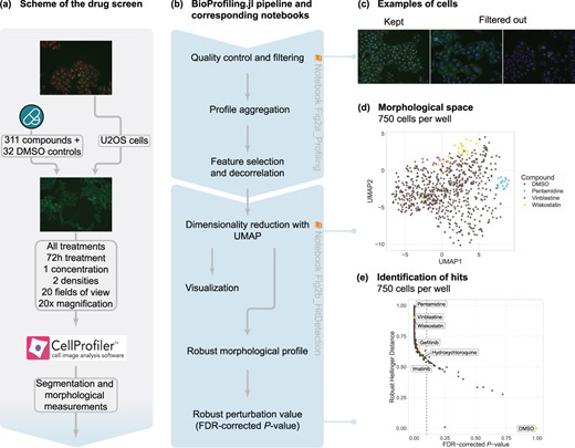
Robust cellular profiling with BioProfiling.jl characterizes the morphological diversity induced by pharmacologically active compounds. (a) Experimental setup of the HCS experiment. Images are uncropped examples of untreated (top) and treated (middle) cells. (b) Computational workflow using BioProfiling.jl. Boxes are annotated with the name of the notebooks with which to reproduce the analyses. (c) Example of images displaying cells kept in the analysis (left) or problematic cells discarded by one of the quality-control filters (center, right). Cytoplasm and nucleus centers are marked with a white cross for each cell. (d) UMAP embedding preserving the cosine distance between the morphological profiles aggregated per field of view in the plate seeded with 750 cells/well. Two out of four dimensions are represented. (e) RHD and RMPV (FDR-corrected P-value) of each compound in the plate seeded with 750 cells/well compared to DMSO. Vertical dotted line indicates an FDR threshold of 0.1 and all compounds on its left are defined as morphological hits

3.2 Investigating curation strategies

The curation of these profiles exemplified a particular set of methodological choices adapted to the specific experimental dataset at hand. BioProfiling.jl does not enforce any single approach and other options could be considered at all steps, from feature selection to dimensionality reduction and quantification of profile distances. As a comparison, we also used one of the other implemented distance metrics, namely the Mahalanobis distance between the center of a perturbation’s profiles and the refence profiles. When no dimensionality reduction was applied, we observed that all profiles were significantly distant from the DMSO. This reflects one consequence of the curse of dimensionality, namely that pairwise distances tend to be similar in high-dimensional spaces (Supplementary Fig. S3a). Using PCA in a strategy analogous to the mp-value (Hutz et al., 2013), we obtained a space where the first axis explained the majority of the data variance, but still displayed some compound clustering (Supplementary Fig. S3b). When comparing the hits obtained with this approach to the initial hit list obtained with UMAP and the RHD (Supplementary Fig. S3c), we observed a partial but significant overlap (Jaccard index of 0.23; ${\chi }^2$ test of independence: P = 1.5e−13). The hits obtained with PCA were only a subset of the hits initially obtained, suggesting that certain morphological changes can be better detected using nonlinear dimensionality reduction techniques. Overall, the choice of methodology has a considerable impact on which perturbations are identified as morphologically active, and consequently on all downstream analyses.

Note that BioProfiling.jl is not only versatile in respect to the profiling approaches, but also supports multiple experimental setups and data types, as any tabular data compatible with the common DataFrame structure can be used as input to define an Experiment object. We provide one additional example from a publicly available dataset using the Cell Painting assay (Bray et al., 2016) to characterize overexpression constructs. By curating and representing profiles for two plates, we observe a visible clustering for some target genes (Supplementary Fig. S4a and b). Overall, comparing the RHD of each target to non-targeting controls correlates well across plates despite processing both plates independently (Supplementary Fig. 4c), which supports the robustness of the chosen approach.

3.3 Exploring MOAs of active compounds

We next went on to characterize the compounds with a strong morphological impact identified on the plate seeded with 750 cells per well using the approach relying on UMAP reduction and RHD. Among the wide range of MOAs covered by the library, 10 hit compounds were known Dopamine receptor antagonists, six hit compounds were annotated to Calcium channel blockers and six to Adrenergic receptor antagonists (Fig.  3a). In this experiment, some MOAs were likelier than others to induce morphological changes, often in accordance with their biological role. In particular, all Tubulin inhibitors caused cytoskeletal defects and were identified as hits. In contrast, only half of the Topoisomerase inhibitors, which modulate DNA replication and transcription and are more likely to impact cell shape indirectly, if at all, were found to modulate the morphology. We note the presence of many oncological and chemotherapeutic agents (PDGFR receptor inhibitors, Topoisomerase inhibitors, KIT inhibitors, Tubulin inhibitors) and neurological drugs (Dopamine receptor antagonists, Tricyclic antidepressants, Norepinephrine reuptake inhibitors) among the morphological hits. Cell shape indeed plays an essential role in cancers, as cancerous cells are typically diagnosed by pathologists based on their morphology. Cell proliferation and several signaling pathways are also associated with cell geometry (Aragona et al., 2013; Dupont et al., 2011; Sero et al., 2015). Some compounds used to treat neurological disorders were also previously reported to induce morphological changes (Wawer et al., 2014), yet the mechanisms linking morphology and disease phenotype are still to be uncovered.

Fig. 3.

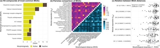
Morphological profiling and data integration characterize compound MOAs. (a) Number of hits and total number of compounds for the most common MOAs in the chemical library. (b) Dissimilarity of the molecular targets on a PPI network (s_AB score, upper triangle) and of the morphological profiles (RHD, lower triangle) for the MOAs with at least two hit compounds. (c) Relation between drug module separation (bins of s_AB scores) and morphological distance (RHD)

3.4 Integrating target properties and morphological profiles

We also compare effects between compounds to further exploit the richness of the morphological profiles. We quantified the similarity between the morphological impact of MOAs by aggregating the mean of the pairwise RHD between their respective hit profiles (Fig.  3b). While each MOA had a distinct signature, Glycogen synthase kinase inhibitors and CDK inhibitors were consistently distant from all other MOAs, hinting that modulation of kinase activity and cell signaling is likely to impact the cellular morphology in broad and distinctive ways as opposed to inducing a particular cytoskeletal defect. The largest changes induced by compounds of these MOAs were impacting shape, intensities and distributions of multiple dyes (Supplementary Table S3). Of note, Kenpaullone is both a CDK inhibitor and a Glycogen synthase kinase inhibitor (Supplementary Table S1) which partly explains the observations shared for both MOAs.

While the morphological profiles are informative by themselves, they are best used by integrating additional information about the perturbations they describe. Here, we used available information on the targets of the compounds to contextualize their molecular environment within the PPI network. We quantified the network separation between the targets of different MOAs via the s_AB score, which was used previously to quantify the separation of disease and drug modules (Caldera et al., 2019; Menche et al., 2015). A positive score is associated with well-separated sets of nodes, whereas a negative score corresponds to an overlap. We found that all the strongest network overlaps between MOAs corresponded to shared drug classes. Tricyclic antidepressants and Norepinephrine reuptake inhibitors corresponded to non-selective monoamine reuptake inhibitors (ATC code N06AA). Serotonin receptor antagonists and Dopamine receptor antagonists both included Antipsychotics (ATC code N05A). PDGFR receptor inhibitors and KIT inhibitors were annotated to the exact same compound, Imatinib mesylate, Pazopanib and Sunitinib, which are all protein kinase inhibitors (ATC code L01E).

When comparing morphological profiles, Histamine receptor antagonists were close to many other MOAs and showed the most striking similarities with selective serotonin reuptake inhibitors and Norepinephrine reuptake inhibitors. All three affected primarily the cell shape (Supplementary Table S3). Of note, Histamine receptor antagonists displayed a consistent level of network similarity with all other MOAs. The s_AB values close to zero reflect in part the spread of their 12 molecular targets on the PPI network, suggesting that generic PPI alteration patterns may correspond to morphological effects that are distinctive, but not unique.

By comparing morphological distances to molecular network separation, we observed that overlapping target modules are associated with more similar morphological profiles (Fig.  3c). The effect does not fully explain morphological variability, which emphasizes the presence of intermediate regulatory processes between genotype and phenotype, and that the disruption of some biological processes is not detectable with general cell shape descriptors as experimental readouts. The quantification of morphological distances between profiles based on the UMAP-reduced space also means that part of the information contained in the original data is lost or distorted. Future development of methodologies leveraging the manifold learned by the UMAP method without the need for an embedding in Euclidean space will further alleviate this limitation. However, our results so far already confirm that there is a general association between the PPI network neighborhood targeted by a compound and their morphological outcome. This could be further explored to systematically link cellular morphology to function in health and disease.

4 Discussion

HCS experiments offer a scalable and cost-efficient way to assess multiple conditions in a single experiment with a rich cellular readout. Assembling morphological profiles to describe these experimental conditions is thus essential and requires dedicated tools for data curation, feature selection, quality control, visualization and quantification of morphologically active perturbations. We implemented these tools in a single open-source software with intuitive and flexible data structures and syntax. We demonstrated by a concrete use case how BioProfiling.jl enables new research and allows the exploration of changes in cellular morphology by easing the analysis of large high-content imaging screens.

As Julia is an efficient programming language and allows parallelization of the computations, BioProfiling.jl can process large datasets in a performant manner. The biggest limitation for analyzing large experiments at the single cell level is currently the memory usage, as the full set of morphological measurements needs to be loaded, which can be an issue on personal computers. This may be improved in the future by using lazy loading and allowing the user to process the data by batches. In regard to profile interpretability, BioProfiling.jl can help identify which features are varying the most, rank features by absolute fold-change when comparing two conditions, highlight correlated measurements and format the data for other tools, for instance to represent the typical cell morphology in a particular condition (Khawatmi et al., 2021; Sailem et al., 2015). Of note, BioProfiling.jl offers a systematic way to define filters for data curation and feature selection. This simplifies the automated definition of these steps and could contribute toward the future development of data-driven feature engineering and machine-learning-powered artifact removal techniques to further streamline the process of morphological profiling.

BioProfiling.jl expands the existing landscape of resources available for biological data analysis, as illustrated in our application where we processed morphological measurements so that they can be integrated with PPIs as well as chemical annotations. The library contributes to the growing package ecosystem for bioinformatics in Julia (Roesch et al., 2021) which ensures that the morphological profiling analyses can be combined in larger projects together with other tasks ranging from sequencing to systems biology (Greener et al., 2020; Heirendt et al., 2017; Zea et al., 2016), and other libraries are conveniently available to integrate these different data types (Zakeri et al., 2018). Julia’s interoperability with other programming languages also makes the onboarding easy for users with prior programming experience who, for instance, might prefer to perform certain tasks in R or Python. This is demonstrated in the provided Jupyter notebooks, with all plots being generated using R’s ggplot2 library (Wickham, 2016) and with the computation of the MCD estimators for robust statistical distances which relies on R’s robustbase package, which in turn calls efficient Fortran routines.

Despite being initially designed and extensively tested for morphological profiling, the ability of BioProfiling.jl to handle large high-dimensional datasets and provide dedicated robust normalization and comparison methods could also be leveraged for other data analyses such as single cell transcriptomics or metabolomics experiments, which also require the curation and transformation of data in tabular format.

To provide an exemplary full use case of the BioProfiling.jl package, we conducted and analyzed a chemical high-content imaging screen for characterizing the effect of small molecules across diverse MOAs. The compounds used in the screen were selected to cover a wide range of morphological activity. While large-scale, hypothesis-free screening of small molecules can offer an unbiased view of the compound types that affect cellular morphology (Bryce et al., 2019; Wawer et al., 2014), our library design enabled us to observe significant changes induced by more than three quarters of the used compounds. At the same time, the focused library design limits the interpretation of MOA enrichment among hits. We observed both commonalities and differences in the effects induced by different MOAs, which alter cellular morphology via different molecular changes, involving cytoskeleton, nucleus and protein relocation (Supplementary Tables S2 and S3). The corresponding morphological profiles were further integrated with the information available about the PPI network properties of the compound targets, which proved to offer complementary views of compound effects and emphasized the role HCS could play in unraveling the relationship between cellular morphology and function.

Acknowledgements

We thank Raphael Bednarsky for discussion and feedback on the library and Daniel Malzl for his feedback on the manuscript.

Funding

This work was supported by the Vienna Science and Technology Fund (WWTF) through projects VRG15-005 (to J.M.) and LS16-060 (to J.M. and L.D.) and by the CNRS (International Research Project SysTact to L.D.). C.W.F. was supported by a DOC-fellowship of the Austrian Academy of Sciences: 25525.

Conflict of Interest: none declared.