A Bayesian framework for high-throughput T cell receptor pairing

Abstract

Motivation

The study of T cell receptor (TCR) repertoires has generated new insights into immune system recognition. However, the ability to robustly characterize these populations has been limited by technical barriers and an inability to reliably infer heterodimeric chain pairings for TCRs.

Results

Here, we describe a novel analytical approach to an emerging immune repertoire sequencing method, improving the resolving power of this low-cost technology. This method relies upon the distribution of a T cell population across a 96-well plate, followed by barcoding and sequencing of the relevant transcripts from each T cell. Multicell Analytical Deconvolution for High Yield Paired-chain Evaluation (MAD-HYPE) uses Bayesian inference to more accurately extract TCR information, improving our ability to study and characterize T cell populations for immunology and immunotherapy applications.

Availability and implementation

The MAD-HYPE algorithm is released as an open-source project under the Apache License and is available from https://github.com/birnbaumlab/MAD-HYPE.

Supplementary information

Supplementary data are available at Bioinformatics online.

1 Introduction

T and B cells rely upon somatically recombined antigen receptor heterodimers to enable their recognition of pathogens and cancerous cells. During development, each naïve T and B cell uniquely recombines and expresses its own antigen receptor [T cell receptors (TCRs) and antibodies, respectively], which are the basis of immune recognition and specificity (Fig. 1A). The overall composition of these heterodimeric receptors is complex due to the subunits of each receptor existing in distinct loci in the genome (α and β chains for the TCR, heavy and light chains for antibodies), multiple possible V and J regions for each receptor chain (and the additional D region for TCRβ and antibody heavy chain) and random nucleotides heterogenously added in the junctions between gene segments (Fig. 1B).

Fig. 1.

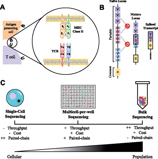
T cell receptor structure, sources of molecular diversity and sequencing methods. (A) T cell receptors (TCRs) are heterodimeric proteins key for immune recognition. The α and β chains each contain constant and variable domains, which form a binding surface that recognizes peptides displayed by major histocompatibility complexes. (B) Each α and β chain generates the molecular diversity required for immune recognition through V(D)J recombination. Additionally, random nucleotides can be added at each junction during formation of the mature receptor chain. The final mRNA transcript combines these components into a single contiguous α or β chain. (C) T cell repertoires can be sequenced through a number of methods. Single-cell methods, such as Drop-Seq or Seq-Well, can retain chain pairing information but typically require physical partitions, which can limit throughput. Bulk sequencing enables high-throughput acquisition of α and β sequences, but lacks the paired-chain information that defines T cell clones. Our discussed form of multicell-per-well sequencing attempts to maintain this throughput while acquiring paired-chain information

Isolating antibodies specific for targets has long been a staple of biotechnology and medicine, allowing for the creation and characterization of molecules ranging from research reagents to FDA-approved drugs. Since the advent of T cell-based immunotherapies as viable cancer treatments in the past several years (Restifo et al., 2012), sequencing of TCRs has seen a similar increase in interest. Moreover, population-level studies of T cell repertoires have produced a number of insightful studies in the last year alone (Dash et al., 2017; Emerson et al., 2017; Glanville et al., 2017).

While antigen receptor sequencing has previously been a laborious process involving the creation of clonal cell lines or sequencing of individual T cells via Sanger sequencing (Dash et al., 2011), the wide adoption of next-generation sequencing has enabled simultaneous sequencing of a large number of immune cells (Fig. 1C). The most straightforward of these approaches involves sequencing antigen receptors from immune cell RNA or gDNA isolated in bulk to gain a repertoire-level understanding of the immune response (Hou et al., 2016). While efficient in accumulating α and β chain sequences, the chain pairings for each clone are forfeited by this approach. Alternative approaches rely on single-cell, partition-based methods to gain high quality paired-chain information such as Drop-Seq (Macosko et al., 2015). In these techniques, single cells are isolated into partitions containing barcodes (e.g. emulsified droplets, microwells), followed by the amplification and sequencing of each chain. Although reliable paired-chain data are produced, cost per sample and limited throughput prevent these methods from becoming ubiquitous. A recently developed method (Howie et al., 2015) merges aspects of bulk and partition-based sequencing to result in a high-throughput procedure with relatively low costs of material and no need for specialized equipment that can recover paired-chain information from immune cell populations.

In this experimental method, multicell-per-well sequencing distributes pools of T cells into individual wells of a 96-well plate. The subpopulation in each well is then simultaneously lysed, reverse transcribed, and amplified with well-specific barcodes. Sequencing of the sample results in lists of α and β chains observed in each well. Analytical methods can capitalize on the co-occurrence of chain pairings across the sample to extract paired-chain information for T cell clones in the original population. This experimental procedure was first described by Howie et al. (2015) using a probabilistic method to score chain pairings. Lee et al. (2017) recently advanced the ability to resolve high-frequency clones using a heuristic scoring algorithm. Our algorithm, termed Multicell Analytical Deconvolution for High Yield Paired-chain Sequencing (MAD-HYPE), describes a new Bayesian approach for the analysis of multicell-per-well sequencing data, improving the identification rates for high-throughput antigen receptor pairing. Moreover, the mathematical framework derived can be readily applied to datasets with variable numbers of cells-per-well in order to further improve receptor pair identification through this emerging sequencing technology.

2 Materials and methods

2.1 Problem overview

The present problem is a pairing task between unique α and β chains in a T cell population. Each cell belongs to a specific clone, defined by its combination of α and β chains, with the following properties:

• Each clone has at least one α chain and one β chain

• Each clone appears multiple times within the population

• Each α or β chain can appear in multiple distinct clones.

In an experiment, the T cell population is observed by distributing a subset of these cells among a specific number of wells, W, which is typically fixed at 96. By lysing, reverse-transcribing, and sequencing the subpopulations in each well, the observer obtains a list of the α chains and β chains present in each well, which can then be used to assign $\alpha \beta$ pairings for clones in the original sample. For justification of the assumptions, see Section 4. An overview of our methodology is shown in Figure 2.

Fig. 2.

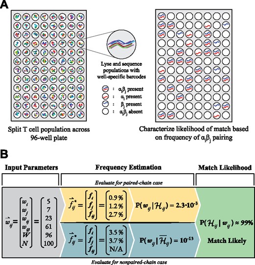
Experimental design and algorithm workflow. (A) Multicell-per-well samples are generated by distributing T cells from a population into each well of a plate (typically with 96 total wells), either through flow cytometry or pipetting. Cells in each well are then lysed, their antigen receptor mRNA transcripts reverse transcribed into DNA, and then amplified with well-specific barcodes. Products from each well can then be pooled and sequenced in order to identify which α and β chains occur in each well. (B) Using this sequencing data, each $\alpha \beta$ combination can be assigned a probability that it exists as a T cell clone. This is achieved through collecting chain-specific parameters, estimating clonal frequencies and observational likelihoods for both paired and non-paired cases, and computing a final match probability

2.2 Bayesian framework

For two chains α_i and β_j, the probability that these chains coexist in a clone, given an experimental observation, is:

$$\mathrm{P}({\mathcal{H}}_{ij}|{\displaystyle \stackrel{\rightharpoonup }{w}})=\frac{\mathrm{P}({\displaystyle \stackrel{\rightharpoonup }{w}}|{\mathcal{H}}_{ij})\mathrm{P}({\mathcal{H}}_{ij})}{\mathrm{P}({\displaystyle \stackrel{\rightharpoonup }{w}}|{\mathcal{H}}_{ij})\mathrm{P}{(\mathcal{H}}_{ij})+\mathrm{P}({\displaystyle \stackrel{\rightharpoonup }{w}}|{\overline{\mathcal{H}}}_{ij})\mathrm{P}({\overline{\mathcal{H}}}_{ij})}$$

(1)

where ${\mathcal{H}}_{ij}$ represents this hypothesis, ${\overline{\mathcal{H}}}_{ij}$ represents the null hypothesis in which these chains do not coexist in any clone and ${\displaystyle \stackrel{\rightharpoonup }{w}}$ are the observed data in the given sample. This is the Bayesian framework we intend to operate on and discuss in the following sections. A complete description of assumptions and observations necessary for the full derivation can be found in the Supplementary Material (Technical Appendix, Section 1).

2.3 Parameterization of sequencing data

After placing a subsample of N cells in each well, a set of unique α and β chains observed over all wells is compiled from the entire sample (N × W cells). As we apply (1) to each possible ${\alpha }_i{\beta }_j$ pairing, we claim the only relevant values from the sample with respect to these two chains are:

• w_ij: the number of wells that contain both α_i and β_j

• w_i: the number of wells that contain α_i but not β_j

• w_j: the number of wells that contain β_i but not α_j

• $w_{Ø}$⁠: the number of wells that contain neither α_i and β_j

• W: the total number of wells in the sample (⁠$w_{ij}+w_i+w_j+w_{Ø}$⁠)

• N: the number of cells allocated to each well.

This collection of parameters is contained in the vector ${{\displaystyle \stackrel{\rightharpoonup }{w}}}_{ij}$ and replaces ${\displaystyle \stackrel{\rightharpoonup }{w}}$ in (1). We assume samples are uniformly distributed between wells, as suggested by Howie et al. (2015), so we may consider only w_ij, w_i, w_j and $w_{Ø}$ and ignore well-specific information.

2.4 Maximum a posteriori estimation of clonal frequency

In order to estimate the probabilities of ${\mathcal{H}}_{ij}$ and ${\overline{\mathcal{H}}}_{ij}$ from ${{\displaystyle \stackrel{\rightharpoonup }{w}}}_{ij}$⁠, we use a latent variable ${{\displaystyle \stackrel{\rightharpoonup }{f}}}_{ij}$ to represent the frequencies of particular collections of clones in the sample. This vector ${{\displaystyle \stackrel{\rightharpoonup }{f}}}_{ij}$⁠, defined for each possible chain pair ${\alpha }_i{\beta }_j$⁠, is composed of three frequencies — f_i, f_j and f_ij — which refer respectively to the frequency of clones with α_i but not β_i, the frequency of clones with β_j but not α_i and the frequency of clones containing both α_i and β_j. We note that f_i and f_j incorporate experimental noise such as premature cell lysis and sequence attrition (e.g. high sequence attrition corresponds to lower f_i and f_j). If evaluating ${{\displaystyle \stackrel{\rightharpoonup }{f}}}_{ij}$ conditioned on ${\overline{\mathcal{H}}}_{ij}$⁠, then f_ij = 0. With these definitions, we can write:

$$\mathrm{P}({{\displaystyle \stackrel{\rightharpoonup }{w}}}_{ij}|{\mathcal{H}}_{ij})={\int \int \int }_T\mathrm{P}({{\displaystyle \stackrel{\rightharpoonup }{w}}}_{ij}|{{\displaystyle \stackrel{\rightharpoonup }{f}}}_{ij},{\mathcal{H}}_{ij})·\mathrm{P}({{\displaystyle \stackrel{\rightharpoonup }{f}}}_{ij}|{\mathcal{H}}_{ij})·d{{\displaystyle \stackrel{\rightharpoonup }{f}}}_{ij}$$

(2)

where $T={[0,1]}^3$ is the domain of ${{\displaystyle \stackrel{\rightharpoonup }{f}}}_{ij}$⁠.

Studies characterizing T cell populations have empirically found that

$$\mathrm{P}({{\displaystyle \stackrel{\rightharpoonup }{f}}}_{ij}|{\mathcal{H}}_{ij})\propto f^{-\alpha }$$

with, for a full T cell repertoire, $\alpha \approx 2$ (Bolkhovskaya et al., 2014). We define α here as the exponent in the probability density function (PDF) for clonal frequency. Some authors, including Bolkhovskaya et al. (2014), have used α for the exponent of the complementary cumulative distribution function (CDF). Both PDF and complementary CDF will follow a power law over a limited range, but exhibit different exponents. By our definition of α, if the set of clonal frequencies is plotted in a log–log histogram (normalized by bar width), the slope will correspond to $-\alpha$⁠. If the cumulative CDF is shown in a log–log plot, its slope will correspond to $-(\alpha -1)$⁠. However, the techniques described here have little sensitivity to this parameter (see Section 4, Discussion). The likelihood function is given by the following:

$$\mathrm{P}({{\displaystyle \stackrel{\rightharpoonup }{w}}}_{ij}|{{\displaystyle \stackrel{\rightharpoonup }{f}}}_{ij},{\mathcal{H}}_{ij})=\left(\begin{array}{c}W\\ {{\displaystyle \stackrel{\rightharpoonup }{w}}}_{ij}\end{array}\right)p_{ij}^{w_{ij}}{p}_i^{w_i}{p}_j^{w_j}{p}_{Ø}^{w_{Ø}}.$$

This multinomial distribution is defined under the derived probabilities:

$$p_{Ø}=(1-f_{i,N})(1-f_{j,N})(1-f_{ij,N})$$

$$p_i=(f_{i,N})(1-f_{j,N})(1-f_{ij,N})$$

$$p_j=(1-f_{i,N})(f_{j,N})(1-f_{ij,N})$$

$$p_{ij}=1-(1-f_{i,N}·f_{j,N})(1-f_{ij,N})$$

where $f_{x,N}=1-{(1-f_x)}^N$ is the probability of clone x being placed in a well with N total cells. This operation is to translate the clonal frequency among cells to the clonal frequency among wells containing N cells. For a complete derivation of these equations, see the Supplementary Material. Integrating (2) numerically over f_ij, f_i and f_j for all ${\alpha }_i{\beta }_j$ pairings quickly becomes intractable for large datasets. However, as this multinomial approaches a multivariate Gaussian distribution, a majority of the probability mass is concentrated near the maximum value. We therefore use a Bayes estimator for ${{\displaystyle \stackrel{\rightharpoonup }{f}}}_{ij}$ based on its posterior distribution given the observed well data ${{\displaystyle \stackrel{\rightharpoonup }{w}}}_{ij}$⁠. Specifically, we use the maximum a posteriori estimator (Robert, 2007) for ${{\displaystyle \stackrel{\rightharpoonup }{f}}}_{ij}$⁠, given by

$${{\displaystyle \stackrel{\rightharpoonup }{f}}}_{ij}^{*}=\underset{{{\displaystyle \stackrel{\rightharpoonup }{f}}}_{ij}\in {[0,1]}^3}{\text{argmax}}\left(\mathrm{P}({{\displaystyle \stackrel{\rightharpoonup }{w}}}_{ij}|{{\displaystyle \stackrel{\rightharpoonup }{f}}}_{ij},{\mathcal{H}}_{ij})·\mathrm{P}({{\displaystyle \stackrel{\rightharpoonup }{f}}}_{ij}|{\mathcal{H}}_{ij})\right)$$

(3)

and we can estimate (2) with

$$\mathrm{P}({{\displaystyle \stackrel{\rightharpoonup }{w}}}_{ij}|{\mathcal{H}}_{ij})\approx \mathrm{P}({{\displaystyle \stackrel{\rightharpoonup }{w}}}_{ij}|{{\displaystyle \stackrel{\rightharpoonup }{f}}}_{ij}^{*},{\mathcal{H}}_{ij})·\mathrm{P}({{\displaystyle \stackrel{\rightharpoonup }{f}}}_{ij}^{*}|{\mathcal{H}}_{ij}).$$

(4)

For conciseness in the equations above, we have designated ${{\displaystyle \stackrel{\rightharpoonup }{f}}}_{ij}^{*}$ as the point estimate for ${{\displaystyle \stackrel{\rightharpoonup }{f}}}_{ij}$ without explicit reference to ${\mathcal{H}}_{ij}$ and ${\overline{\mathcal{H}}}_{ij}$⁠, although this condition does change the estimate (see Supplementary Material, Technical Appendix, Section 1.2). In order to determine $\mathrm{P}({{\displaystyle \stackrel{\rightharpoonup }{w}}}_{ij}|{\overline{\mathcal{H}}}_{ij})$⁠, we simply set f_ij = 0 and repeat the same approach. Once we have estimated $\mathrm{P}({{\displaystyle \stackrel{\rightharpoonup }{w}}}_{ij}|{\mathcal{H}}_{ij})$ and $\mathrm{P}({{\displaystyle \stackrel{\rightharpoonup }{w}}}_{ij}|{\overline{\mathcal{H}}}_{ij})$⁠, the values are input into (1) to acquire a Bayesian estimate of match probability between the given α_i and β_j chain. The priors $\mathrm{P}{(\mathcal{H})}_{ij}$ and $\mathrm{P}({\overline{\mathcal{H}}}_{ij})$ are set to $\frac{1}{n}$ and $\frac{n-1}{n}$⁠, where n is an average of the number of unique α chains and the number of unique β chains observed in the sample. We treat chain creation as an effectively random process during T cell development, and we do not apply any bias toward or away from particular $\alpha \beta$ pairings.

2.5 Data collision adjustment

The previously described Bayesian estimate computes the probability of a particular chain pairing by analyzing every potential chain pairing independently. However, in some cases, clones with similar frequencies in the T cell population can introduce an additional source of error to our predictions. In this subsection, we describe a filter to avoid making predictions under particular error-prone conditions.

We aim to provide an upper bound δ for the false detection rate (FDR) of our predictions due to dependency between chain pairings. To motivate the following analysis, consider two unique clones occupying the same k wells, out of W total wells. Although both pairs ${\alpha }_1{\beta }_1$ and ${\alpha }_2{\beta }_2$ may be correctly identified as pairs, ${\alpha }_1{\beta }_2$ and ${\alpha }_2{\beta }_1$ will share equivalently good match probabilities. The analysis in the previous sections does not account for this additional source of error because it estimates pairing probabilities without regard to other predicted chain pairings. For x clones occupying the same wells, the success rate of identification is bounded by $\frac{1}{x}$⁠, regardless of algorithm scoring. Data sets with more clones over the same frequency range will have increased the error rates due to this effect. This error is mitigated, however, by the vast permutation space. We therefore use the initial distribution of unique α and β chains to define a pre-conditioned success rate filter:

$$1-\frac{1}{(m-1)p+1}<\delta \hspace{1em}\hspace{0.17em}\text{for}\hspace{0.17em}\hspace{1em}\mathrm{p}=\frac{1}{\left(\begin{array}{c}W\\ k\end{array}\right)}$$

where m is the number of clones occupying the same number of wells k.

If this constraint fails for any chain pair occupying k wells, this potential pair is not evaluated to prevent the FDR from being inflated. These boundaries justify limits empirically constructed in previous studies (Howie et al., 2015). A full derivation is included in the SI (Technical Appendix, Section 2).

2.6 Variable cells-per-well

One of the advantages of defining this algorithm within the given framework is that it provides a principled route to analyze data from samples with a variable number of cells in each well. This is heuristically studied by Lee et al. (2017), but we can rigorously define a general algorithm for these cases. To begin, we still parameterize our data set, but we now break each parameter into P partitions, where P is the number of sets of wells with a distinct number of cells-per-well. This changes ${{\displaystyle \stackrel{\rightharpoonup }{w}}}_{ij}$ into a vector of vectors ${{\displaystyle \stackrel{\rightharpoonup }{w}}}_{ij,p}$⁠, each containing $w_{ij},\hspace{0.17em}{w}_i,\hspace{0.17em}{w}_j,\hspace{0.17em}{w}_{Ø}$⁠, W and N. This is integrated into the algorithm by modifying (3) and (4):

(5)

$$\mathrm{P}({{\displaystyle \stackrel{\rightharpoonup }{w}}}_{ij}|{\mathcal{H}}_{ij})\approx \mathrm{P}({{\displaystyle \stackrel{\rightharpoonup }{f}}}_{ij}^{*}|{\mathcal{H}}_{ij})·\prod _{p=1}^P\mathrm{P}({{\displaystyle \stackrel{\rightharpoonup }{w}}}_{ij,p}|{{\displaystyle \stackrel{\rightharpoonup }{f}}}_{ij}^{*},{\mathcal{H}}_{ij}).$$

(6)

Together, these modifications are used to predict pair probabilities on any experimental distribution of cells across wells.

2.7 Experimental and simulated datasets

Experimental datasets were taken from Howie et al. (2015) in order to demonstrate ability to recover paired-chain information in biological contexts. To validate the performance of the algorithm over diverse parameter ranges, simulated T cell repertoires were used. Each dataset was initialized using a set number of unique clones, n, and a distribution of clonal frequencies. For the power-law distribution, observed previously in T cell populations (Bolkhovskaya et al., 2014), two parameters were specified: a constant α that produced the relationship for the clonal frequency $P(f_{ij})\propto f^{-\alpha }$⁠, and the maximum observed frequency in the population, $f_{\text{max}}$⁠. For uniform distributions, as used in computational studies of T cell sampling (Sepúlveda et al., 2010), the frequency was simply set to $\frac{1}{n}$⁠. To generate sequencing datasets from a simulated repertoire, clones were randomly distributed according to the number of declared wells and cells-per-well. To mimic experimental samples, sequence attrition was added, in which any chain in a well had a fixed probability of decaying independently of other chains in the well, and a chain misplacement probability, in which a chain in a well has a set probability that it randomly migrates to another well in the sample. The final result was an anonymized list of α and β chains that were successfully observed in each well of a sample.

2.8 Implementation

The MAD-HYPE algorithm is implemented in Python 2.7, and is publicly available at https://github.com/birnbaumlab/MAD-HYPE. Computation time scales as $O(n^2)$ with the total number of observed chains because each pair of unique α and β chains is evaluated independently. We applied parallel computing and the data collision adjustment filter, which renders a substantial number of observed clones irrelevant to analyze when searching for matches, to improve computation time.

3 Results

3.1 Performance on simulated datasets

In order to assess the performance of the MAD-HYPE algorithm across diverse parameter ranges, datasets were generated that resembled physiologically relevant clonal populations. Figure 3 demonstrates our algorithm on a simulated clonal repertoire, generated using a power-law distribution with $\alpha =2.0$ (Bolkhovskaya et al., 2014), a sequencing error attrition rate of 10%, consistent with Howie et al. (2015), and a maximum clonal frequency of 1%. The relationship between ${{\displaystyle \stackrel{\rightharpoonup }{w}}}_{ij}$ and the chain pairing probability $\mathrm{P}({\mathcal{H}}_{ij}|{{\displaystyle \stackrel{\rightharpoonup }{w}}}_{ij})$ is shown, along with other identification metrics for this simulation. For future simulations, we refer to two main performance metrics:

1. Clonal matches—the number or percentage of correct $\alpha \beta$ matches made at the given FDR

2. Repertoire coverage—the sum of frequencies for correct matches made at the given FDR.

Fig. 3.

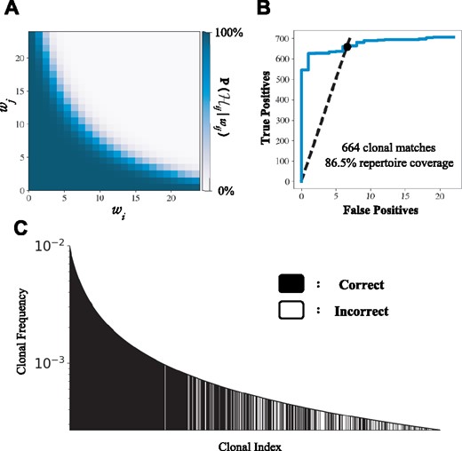
Demonstration of MAD-HYPE performance. (A) Simulated chain pair probabilities, where w_ij is fixed at 24. When $w_i$ and $w_j$ are kept low, it becomes exceeding unlikely for 24 wells to coincidentally have both α_i and β_j, which produces a high match probability. As $w_i$ and $w_j$ increase, it becomes increasingly likely to observe w_ij due to chance. (B) Paired-chain identification for simulated dataset. A repertoire of 1000 clones was simulated with clonal frequencies following a power-law distribution. 100 cells were allocated into each of 96 wells, with a sequence attrition rate of 10%. At an FDR of 1%, 664 clonal matches were identified, representing 86.5% repertoire coverage. (C) Alternative representation of simulation performance. Each band represents a clone with a given frequency, with black indicating whether the pairing was successfully identified. Clonal index refers to the clone’s position in a list ordered by decreasing frequency

For this particular simulation, 664 out of 1000 clonal matches were made, and a repertoire coverage of 86.5% was achieved, both at a FDR of 1%. If unstated, subsequent studies on simulated data are performed using these default parameters.

Compute times required for analysis of selected experimental and simulated datasets are shown in Supplementary Tables S1 and S2.

3.2 Variable cell-per-well counts

With the application of the Bayesian system defined in (6), we explored the ability of the MAD-HYPE algorithm to deconvolute chain pairings from samples explicitly designed to have a varying number of cells-per-well. To highlight the effect this experimental parameter can have on chain pair identification, we fixed the number of cells in the sample at 96 000 and defined two partitions of a 96-well plate. The number of wells and cells-per-well is set for one partition, and implicitly solved for in the other partition, so as to add up to the total cell count. The repertoire coverage is shown for this demonstration in Figure 4A. Three distinct parameter sets are shown in Figure 4B–E, which illustrate the effects of different experimental design choices. Predicted frequency refers to f_ij solved for in (5).

Fig. 4.

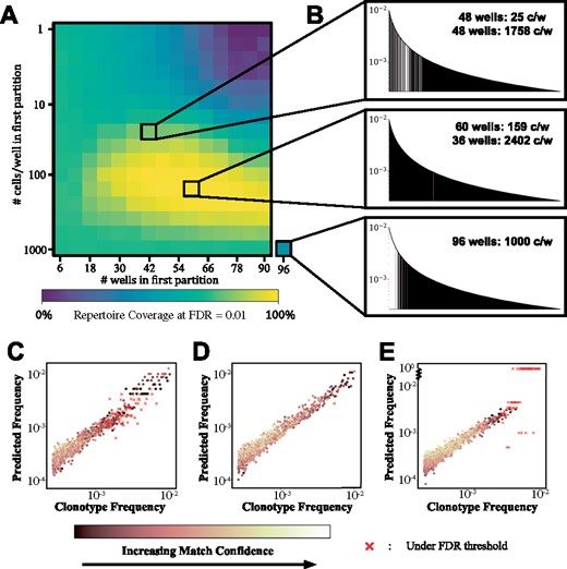
Application to samples with variable cells-per-well. (A) An advantage of MAD-HYPE is the ability to easily extend its function to experiments designed with a variable number of cells-per-well. Here, we consider simulated repertoires with samples containing a constant number of total cells (96 000 cells per sample). These cells are allocated in two distinct partitions, each with a subset of wells and set number of cells-per-well. Axes indicate the first partition’s number of wells and cells-per-well, after which all remaining cells are distributed uniformly among the remaining wells. (B) Three different experimental designs featuring different partitioning strategies illustrate the variety of effects that can be produced. If partitions have their cell-per-well counts spread too far apart (B, top), mid-frequency clones cannot be resolved (C). If partitions are designed with appropriate cell-per-well counts (B, middle), clones with wide ranges of frequencies can be successfully identified (D). If only one partition is made (B, bottom), the algorithm performs well on a subset of frequencies. In this case, high-frequency clones now fail to be resolved (E)

3.3 Sensitivity to experimental noise

We aimed to assess the sensitivity of our methodology to a number of parameters used throughout the study. First, we ran simulations in which we varied the noise parameters for chain deletion (Supplementary Fig. S1A and B) and chain misplacement (Supplementary Fig. S1C and D). Although performance did decay as noise magnitude increased, observed noise ranges of chain deletion (˜10%, Howie et al., 2015) showed minimal loss in clonal match count and repertoire coverage. Chain misplacement probability had a steeper effect on clonal matches and repertoire coverage, although we note this form of experimental noise is typically lower than chain deletion.

3.4 Sensitivity to dual clones and chain sharing

During the T cell recombination process, both chromosomes can produce functional TCRα and TCRβ loci. This can result in two unique α and/or β chains existing within a single clone. Mature cells exhibiting this characteristic, termed dual clones, are observed at a rate under one-third for α chains (Padovan et al., 1993) and 6–7% for β chains (Eltahla et al., 2016; Stubbington et al., 2016). Simulations incorporating this property into MAD-HYPE demonstrate a resilience to change in both clonal match count and repertoire coverage (Supplementary Fig. S2A and C). A similar confounding factor to T cell pairing is chain sharing, or the event in which multiple clones share an identical α chain or β chain in a repertoire. This process was experimentally addressed in Lee et al. (2017) where they devised a clonal sharing structure that mimicked experimentally observed distributions. The same structure was included in MAD-HYPE simulations. While a loss was observed in performance (Supplementary Fig. S2B and D), MAD-HYPE was still able to retain a significant degree of repertoire identification.

3.5 Sensitivity to repertoire architecture

Simulations discussed thus far have primarily used T cell populations defined through a power-law distribution with α = 2. Although this value was chosen to mirror experimental distributions (Bolkhovskaya et al., 2014; Sherwood et al., 2013; Zheng et al., 2017), there exist cases where this parameter may span different values. For example, a heavily expanded population of isolated T cells responding to a particular antigen may possess a distribution with an α larger than 2. As such, we performed analysis on simulated repertoires with α ranging from 1.5 to 3, with and without chain sharing (as defined by Lee et al., 2017). These results are shown in Supplementary Figure S3, where we find our methodology stands for reasonable ranges of α. We also tested the algorithm on uniform repertoire distributions, in which all clones have equal clonal frequency (Supplementary Fig. S4A and B). MAD-HYPE remained effective within a moving bandwidth which illustrated a positive correlation between the number of cells per well and the clonal frequencies successfully paired. We note any failure to identify clones generally does not result from MAD-HYPE being pre-disposed to solving certain architectures, but rather to resolving certain clonal frequencies. As α is changed, the frequencies present in the repertoire similarly change, which forces frequencies out of the resolving range for the given number of wells and cells-per-well.

Lastly, we tested for sensitivity to the prior parameter, α. Despite covering two orders of magnitude in parameter value, insignificant changes were observed in performance (Supplementary Fig. S4C and D). We refer here to the α used to define the frequency prior in (2). This differs from the α referred to previously in this subsection, which describes the true power-law distribution for a repertoire of simulated clonal frequencies.

3.6 Comparison to pairSEQ algorithm

Multicell-per-well sequencing was first analytically framed by Howie using a probabilistic framework (Howie et al., 2015). In order to validate their approach, two patients, X and Y, had a subset of their T cell repertoire isolated. Each population was genomically sequenced to provide a reference for which patient each α and β chain originated from. Samples from the patients were then mixed and distributed into 96-well plates, and deep sequenced for downstream analysis. An implementation of their algorithm and code base was not available. Therefore, we compared our methodology by using MAD-HYPE on Howie et al. (2015) sequencing data and aligning our performance to their published results. We chose to focus on their first and second experiment since these experiments contained a true reference that could be used to estimate FDR by labeling predicted matches as either true positives or true negatives. We note that the number of positives/negatives deviates slightly (<3%) from the published values due to lack of reported hyperparameters defining sequence data interpretation. However, this does not affect the total number of matches reported at the given FDR.

The results for each of these are shown in Figure 5A. α chain and β chain repertoires were first sequenced from each subject, so that true positives (α/β chains originating from subject X/X or Y/Y) and true negatives (α/β chains originating from subject X/Y or Y/X) could be used to estimate the FDR. Furthermore, this ratio can be used to estimate the FDR for the total number of matches that could be made in a sample, inclusive of matches with ambiguous origin. This metric is independent of repertoire overlap and the mapping of chain to subject. For this reason, total matches are the most appropriate estimation of algorithm performance given this experimental design. The two experiments shown have a different number of cells-per-well (2000 and 80 000 per subject, respectively) to help demonstrate the scales at which the system can operate. In Experiment 1, 4 933 $\alpha \beta$ total matches were identified from subjects X and Y at an FDR =1%. In Experiment 2, 176 366 clonal $\alpha \beta$ total matches were identified from subjects X and Y. The MAD-HYPE algorithm increased the identification rate of clonal pairings relative to pairSEQ by 19.1 and 13.2% in Experiments 1 and 2, respectively.

Fig. 5.

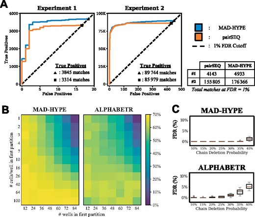
Comparison to existing multicell-per-well algorithms, pairSEQ (Howie et al., 2015) and ALPHABETR (Lee et al., 2017). (A) Comparison of performance of MAD-HYPE to results disclosed by Howie et al. (2015). Data were taken from Experiments 1 and 2, in which full repertoires were sequenced from two patients, X and Y, at two different cell-per-well counts (2000 and 80 000, respectively). MAD-HYPE was used to identify chain pairings, and the results were compared to those disclosed in the Supplementary Material of Howie et al. (2015). We note that each false positive detected (X/Y and Y/X) accounts for two estimated false positive events due to the randomization of chain origin. (B) Heatmaps show repertoire coverage of MAD-HYPE and ALPHABETR using simulated repertoires comparable to physiological samples (1000 clones, power-law clone frequency distribution, $\alpha =2.0,\hspace{0.17em}{f}_{\text{max}}=1\%$⁠). Column and row labels are interpreted the same as in Figure 4a, but with a total of 9600 cells over all 96 wells. Chain sharing probabilities proposed by Lee et al. (2017) were used. Each data point is an average of 10 simulations. (C) FDR for varying chain deletion probability over the top 250 predicted matches for MAD-HYPE and ALPHABETR, using 1000 clones, 300 cells-per-well, and chain sharing proposed by Lee, averaged across 10 simulations. More cutoffs can be observed in Supplementary Figure S6

3.7 Comparison to ALPHABETR algorithm

An alternative algorithm, ALPHABETR (Lee et al., 2017), uses a heuristic method to score chain pairs coexisting in wells. Performance was compared over a similar parameter range as in Figure 4A, but with 9600 cells per sample for an average of 100 cells-per-well over the 96-well plate (Fig. 5B). In the region of high performance (cell-per-well counts between 40 and 100, partition sizes between 12 and 36), MAD-HYPE outperforms ALPHABETR in repertoire coverage by an average of 5 percentage points. In general, ALPHABETR successfully identifies more high-frequency clones, while MAD-HYPE identifies more low-frequency clones (Supplementary Fig. S5). This discrepancy causes ALPHABETR to sometimes outperform MAD-HYPE in repertoire coverage despite identifying fewer clones. Because clonal frequencies are distributed following a power law, there will be a greater number of clones with low frequencies than with high frequencies, so MAD-HYPE is more effective at identifying a greater fraction of the clones present in a repertoire. However, ALPHABETR has higher FDR in many cases. We observe the FDR of match guesses made with highest ranked confidence in each algorithm in Figure 5C, and continued in Supplementary Figure S6. These simulations were performed with 300 cells-per-well and chain sharing probabilities proposed by Lee.

3.8 Experimental design recommendations

The proposed algorithm contains a predictable relationship between the number of cells placed in each well and the clonal frequencies identified (Supplementary Fig. S4A and B); in general, the MAD-HYPE can be tuned to identify clones of any frequency by adjusting these cell-per-well counts. That is, the appropriate cell-per-well counts depend on the clonal frequencies of interest. For instance, if high-frequency clones are of interest, then low cell-per-well counts are necessary. Low-frequency clones are identifiable using high cell-per-well counts.

Variable cells-per-well can be used to broaden the resolvable frequency band. To help illustrate how to use variable cells-per-well in sample dependent ways, we aimed to provide recommendations for experimental design based on sample type. We drew parameters from literature for peripheral blood samples (Bolkhovskaya et al., 2014) and lymphocytes isolated from tissues (Zheng et al., 2017). For peripheral blood simulations, we divided a 96-well plate into two partitions with 500 and 10 000 cells-per-well. When the diversity of the T cell repertoire is high, 95.7% of the simulated repertoire was identified (Supplementary Fig. S7A). When the repertoire is less diverse, 68.4% of the repertoire was identified (Supplementary Fig. S7B). For tissue-derived samples, repertoires were fit to data from Sherwood et al. (2013) and Zheng et al. (2017). In these cases, >99% of repertoire was identified for samples with two 48-well partitions, while using 50 and 1000 cells-per-well (Supplementary Fig. S7C and D).

4 Discussion

We have described here a new computational method to identify TCR$\alpha \beta$ pairings using subsampled T cell populations. Moreover, we have focused on how to objectively design experiments to expand the clonal frequency range identified in an experiment by varying the number of cells-per-well. Additionally, we have described a number of usage cases for the MAD-HYPE algorithm which outperforms existing standards for paired-chain identification in multicell-per-well repertoire sequencing experiments. For biological samples taken from Howie et al. (2015), there are modest improvements in clonal match count. In addition, we note a few key differences between MAD-HYPE and pairSEQ:

• pairSEQ requires the approximation of error rates in samples by an additional experimental procedure, which is not required by MAD-HYPE (Howie et al., 2015)

• Significant effort was put forward to make methodology transparent, and implementation is available at: https://github.com/birnbaumlab/MAD-HYPE

• The framework established here can be adapted to a more robust collection of experimental designs, such as variable cells-per-well, which shows dramatically improved efficacy in repertoire identification (Fig. 5A).

Using simulated data, we found MAD-HYPE to outperform ALPHABETR under most experimental conditions. We observed the following important performance differences:

• The computation time to perform MAD-HYPE analysis on a sample scales as $O(n^2)$ with the number of observed chains. ALPHABETR, which internally uses the Hungarian algorithm (Kuhn, 1955) to match α and β chains within each well, scales as $O(n^3)$ with the number of unique chains per well. For large repertoires with experimentally observed skews, we expect the number of unique chains per well to be approximately proportional to the total number of observed chains. Thus, MAD-HYPE will be computationally feasible for larger samples than ALPHABETR. See Supplementary Figure S8 for side-by-side comparison of computation times.

• MAD-HYPE consistently performed better at identifying low-frequency clones, while ALPHABETR was more effective at identifying high-frequency clones (Supplementary Fig. S5). We note that multicell-per-well algorithms are generally of interest for identifying high numbers of low-frequency clones, and that identification of high-frequency clones may be better suited to more conventional single-cell sequencing approaches.

• MAD-HYPE consistently identified more clonal matches. However, under some conditions, ALPHABETR achieved greater repertoire coverage because it identified more high-frequency clones (Supplementary Fig. S5).

• ALPHABETR’s scoring heuristic causes many chain pairs to be equally scored with the highest possible score. This lack of resolution at the top of scoring range prevents fine-tuned choice of the most certain clones, which may be desired in cases where the set of all top-scoring chain pairs already surpasses the FDR.

One of the central challenges to this methodology is trying to limit experimental noise. Each cell placed into a well ideally releases mRNA for both chains, which is identified after sequencing. However, if one of these chains evades detection and the other is successfully sequenced, the algorithm will lower the probability of a match between this pairing since there are wells that lack coexistence. Therefore, any experimental efforts to minimize this attrition rate are paramount. Although sensitivity was only moderate (Supplementary Fig. S1), minimization of this is likely the largest technical hurdle to large-scale application. We also note that we did not include noise sources representing cell death, or other effects that delete all chains of a clone simultaneously. Adjustments can be easily made to counter this effect (e.g. if 50% of cells perish before sequencing, simply allocate twice the number of cells as intended to each well initially).

We note that while T cells only utilize one recombined TCR α chain and β chain pairing to recognize any given antigen, it is possible for a T cell to contain a second V(D)J-recombined α or β chain that can confound analysis. While these ‘extra’ chains, which arise from recombination events that were insufficient for the T cell to pass thymic selection, can often be computationally filtered out of the data set (e.g. when one of the recombination events does not produce an in-frame transcript), there are also cases where the identity of the functional chain cannot be computationally determined. Even though functionally resolving these ambiguities is challenging for any sequencing technique, this does not affect computational analysis: a T cell containing one β chain but two α chains would be regarded as two independent pairing events. If a researcher wished to further resolve the functional chain pairing, they could either cross-reference putative pairs with other T cells in the sample (since a functional chain in an antigen-experienced T cell pool is more likely to share homology with other sequences), or functionally test the potential pairings.

Moreover, any multicell-per-well sequencing experiment is restricted to the identification of clonal pairings that occur in multiple cells across the sample. Since resolving clones relies exclusively on observing $\alpha \beta$ pairings multiple times throughout a sample, one instance is never sufficient. Although potentially limiting, in practice most T cell populations are expanded to some degree, ensuring a majority of available clones have numerous copies in any given sample.

As illustrated previously (Fig. 4), there exists a trade-off between the number of cells-per-well and the ability to resolve clones at a certain frequency. If there are too few cells-per-well, low-frequency clones appear too infrequently to provide a permutation space with adequate sparsity. Likewise, if too many cells are allocated in each well, high-frequency clones will appear in every well, again producing collisions in permutation space. In Figure 4C, the resolving power of MAD-HYPE for each partition is discontiguous, allowing the identification of clones at only high and low frequencies, and failing to identify mid-frequency clones. In Figure 4E, a single partition enables the accurate identification at mid- and low-frequency clones, but fails to enable the identification of high-frequency clones. Moreover, MAD-HYPE predicts these clones to have $f_{ij}=100\%$ because they appear in all wells of the sample. If the partitions are designed correctly, as in Figure 4D, high resolving power can be maintained throughout the entire spectrum of frequencies in the sample without modifying the total number of cells employed.

This highlights a critical point of multicell-per-well experimentation: the choice of the number of cells-per-well has a direct impact on the clonal frequencies that can be resolved. This is particularly important in the case of partitioned samples, where each set of wells at a specific number of cells-per-well resolves a certain bandwidth of clonal frequencies. This property is evident in both Supplementary Figures S4C and D and S9, illustrating approximate regimes where this occurs. The recommendations for sample type are derived from this property because well partitions should be chosen to create contiguous frequency ranges in which clones can be resolved. Careful attention should be paid to this choice during experimental design, when the user may consider which clonal frequencies will be of greatest value. If the high-frequency clones in a sample are of greatest interest, a low number of cells-per-well should be used. Conversely, if a study requires the characterization of thousands of low-frequency clones, a higher cell-per-well count should be used.

The resolving power can be increased by choosing more partitions at finer-grain resolution than that shown in Figure 4. However, optimizing such a setup becomes computationally intractable to rigorously solve, as the parameter space increases by two for each added partition (W_p, N_p) and less robust as these parameters are fitted closer to the predicted repertoire characteristics and prior distributions. We therefore leave this topic as an accessible, but sample dependent, problem that can be solved at the user’s discretion. The recommendations made through Supplementary Figure S7 stand as an approximate experimental design to start from.

While this study has focused primarily on the application to sequencing T cell repertoires, this methodology can be directly applied to many other contexts. A direct parallel would be the sequencing of γδ T cell populations, in which one would identify chain pairings between TCRγ and TCRδ chains, rather than between TCRα and TCRβ chains. Similarly, B cell populations could be sequenced to identify pairings between heavy and light chains. In general, any sample that contains two spatially separate transcripts with variable regions is a sufficient condition to use MAD-HYPE in order to recompose original clonal characteristics.

5 Conclusion

The progress documented here represents a new algorithmic approach to resolve paired-chain sequencing data from multicell-per-well sequencing experiments. Our approach has been validated in the context of simulated datasets drawn from observed parameters, as well as on experimental samples taken from Howie et al. (2015). Our performance exceeded that of existing methodologies (Fig. 5) and can be readily applied to new experimental designs that were previously unapproachable in a non-heuristic format (Fig. 4). Future extensions of MAD-HYPE could involve additional analysis to identify clones of the T cell population with two α and/or two β chains, rather than only identifying $\alpha \beta$ pairings. The direct application of our methodology to this problem is discussed in the Supplementary Material (Technical Appendix, Section 1.4). As sequencing power grows and we aim to characterize full T cell repertoires, MAD-HYPE and similar algorithms represent a robust technique with the potential to lower technical thresholds while maintaining throughput.

Acknowledgements

We would like to acknowledge Paul Blainey and Michael Yaffe for their feedback during algorithm development.

Funding

Funding for P.V.H. and J.B. was provided by the National Science Foundation Graduate Research Fellowships Program. Funding from the National Science Foundation Physics of Living Systems (PHY-1305537 and PHY-1707999 to J.B. and M.B.) is gratefully acknowledged. Additional funding was provided through National Cancer Institute [P30-CA14051] and fellowships from the Packard Foundation, the V Foundation and the AACR-TESARO Career Development Award for Immuno-oncology Research [17-20-47-BIRN] for M.E.B.

Conflict of Interest: none declared.

Author notes

The authors wish it to be known that, in their opinion, the first two authors should be regarded as Joint First Authors.