


Abstract
Bacterial infections are a major cause of illness worldwide. However, most bacterial strains pose no threat to human health and may even be beneficial. Thus, developing powerful diagnostic bioinformatic tools that differentiate pathogenic from commensal bacteria are critical for effective treatment of bacterial infections.
We propose a machine-learning approach for classifying human-hosted bacteria as pathogenic or non-pathogenic based on their genome-derived proteomes. Our approach is based on sparse Support Vector Machines (SVM), which autonomously selects a small set of genes that are related to bacterial pathogenicity. We implement our approach as a tool—‘Bacterial Pathogenicity Classification via sparse-SVM’ (BacPaCS)—which is fully automated and handles datasets significantly larger than those previously used. BacPaCS shows high accuracy in distinguishing pathogenic from non-pathogenic bacteria, in a clinically relevant dataset, comprising only human-hosted bacteria. Among the genes that received the highest positive weight in the resulting classifier, we found genes that are known to be related to bacterial pathogenicity, in addition to novel candidates, whose involvement in bacterial virulence was never reported.
The code and the resulting model are available at: https://github.com/barashe/bacpacs.
Supplementary data are available at Bioinformatics online.
1 Introduction
According to the World Health Organization, infectious diseases are still one of the top causes of death globally. This is despite the advance of modern medicine in the post-antibiotic era. Recently, it became clear that humans are heavily colonized by thousands of different microbial species, overall called microbiota, which are either innocuous or beneficial to human health. For example, gut microbiota are important for nutrition, development and regulation of the immune response (Hooper and Gordon, 2001; Qin et al., 2010).
As the core microbiota of humans is largely diverse, the determination of whether a specific bacterial strain is commensal or pathogenic to humans is extremely challenging. In addition, commensal human bacteria can evolve into pathogenic bacteria by acquisition of novel genes via the horizontal gene transfer (HGT) mechanism (Kelly et al., 2009; Soucy et al., 2015). This complicates clinical diagnosis, which uses traditional methods, and encourages using complete genome sequencing to reveal new genetic traits. It also motivates the need to identify human-pathogenic (HP) strains, and to understand their virulence mechanisms; such studies could facilitate the identification of contaminated food, increase the accuracy of infection diagnosis, provide better patient treatment and lead to a better development of targeted drugs and vaccines.
In current clinical practices, the determination of an infection agent is based on Koch’s postulates, established in the 19th century. These require animal models and methods to isolate bacterial strains and culture them (Sassetti et al., 2003; Young et al., 1985). However, many pathogens are human-specific and therefore cannot infect animals, making the identification of infection agents highly challenging.
Due to recent advances in next-generation sequencing (NGS) technologies, many new databases that contain the available bacterial sequences have been created and their data are accumulating rapidly (Benson et al., 2015; Kulikova et al., 2007; Mashima et al., 2016; O’Leary et al., 2016). To date, complete genome sequences of almost all major bacterial pathogens have been determined, providing significant insights into microbial pathogenesis. In addition, several repositories that collect virulence factors and annotate their structures, functions and mechanisms, are available (Chen et al., 2005; Zhou et al., 2007). Furthermore, sequences of non-human pathogenic (NHP) bacteria, such as microbiome species, are also collected and deposited in sequence databases (Chen et al., 2010, 2017; Gevers et al., 2012). Altogether, the number of available sequenced bacterial genomes is at the range of hundreds of thousands and is growing rapidly (Mashima et al., 2016; O’Leary et al., 2016).
The theme of this paper is a new machine-learning approach for classifying human-hosted bacteria as HP or NHP, based on their proteomes. A tool, developed based on this approach, could be used for future surveillance of food- and water-borne pathogens, as whole-genome sequencing of food products and water sources is gradually becoming a standard (Carleton and Gerner-Smidt, 2016). Currently-available tools for pathogenicity prediction can broadly be divided into two classes: protein-content based (Andreatta et al., 2010; Cosentino et al., 2013; Garg and Gupta, 2008; Iraola et al., 2012) and read based (Byrd et al., 2014; Deneke et al., 2017; Naccache et al., 2014). The approach we propose in this paper belongs to the former category. The existing tools for each category are reviewed below. Comparative analysis of Bacterial Pathogenicity Classification via sparse-SVM (BacPaCS) versus the most recent tool in each category is given in Section 3.4.
Protein-content based approaches require the availability of assembled genomes and characterize the phenotype of a microbe by the presence/absence of members of protein families (PFs) in its genomes. Such methods have great potential not only for prediction but also for qualitative analyses [e.g. identifying clade-specific proteins that are either positively or negatively correlated with a pathogenic phenotype (Cosentino et al., 2013)]. Furthermore, some of the methods in this category utilize the complete coding information and are thus able to discover novel unannotated proteins that contribute to bacterial virulence (exemplified in Section 3.3). Their drawbacks are in the dependence on genome assembly and annotation, and in neglecting the signal potentially found outside of the protein-coding sequences.
The first tool in this category was developed by Garg et al. (Garg and Gupta, 2008) and used a cascade Support Vector Machines (SVM) classifier (Graf et al., 2004) to predict whether a given bacterial protein is associated with bacterial virulence. Another method, developed later by Iraola et al. (Iraola et al., 2012), proposed an SVM model to predict bacterial virulence, using known families of orthologous genes. Both of these methods (Garg and Gupta, 2008; Iraola et al., 2012) relied on pre-established databases of virulence factors, that annotate virulence at the gene level, and were therefore limited to specific proteins that are known to be involved in virulence. In contrast, many unannotated genes, whose sequences are available and potentially associated with virulence (or anti-virulence) function, were overlooked by these tools.
Other protein-content based tools for pathogenicity prediction were developed without using pre-established PFs, but rather by creating PFs and annotating them, based on their appearance frequency in pathogenic or non-pathogenic organisms (Andreatta et al., 2010; Cosentino et al., 2013). These studies required an initial step, where proteins of all organisms in the training set were clustered to form PFs. PFs significantly enriched in either HP or NHP were assigned a weight value, depending on the degree of the enrichment, while families that were not significantly enriched were discarded. To determine the pathogenicity of a new bacterial strain (not found in the training set) its protein sequences were aligned against the PFs, and a score was computed according to the presence or the absence of PFs that are known to be enriched in HP or NHP.
While these methods were novel in not relying on previously known PFs, they required manual selection of PFs that are significantly enriched in HP, therefore these PFs were specific to the chosen dataset. In addition, both methods were trained on datasets that included bacterial species that were never detected in human samples, therefore their biological relevance to human diseases was questionable. Finally, all methods were designed based on the genomic data available at the time, but unfortunately cannot be scaled up to the increasing volume of genomic data that are quickly becoming available. This is due to the computational bottleneck of the first step: clustering proteins into PFs.
Here, we propose a novel approach that overcomes the above limitations by being fully automated, trained only on clinically relevant data (containing human commensal and pathogenic bacteria), and implements a clustering method that considerably shortens the computation time, making it practically more relevant. This is discussed in detail in Section 2.2.
Read-based classification approaches use short genomic reads as raw input. Several tools were proposed for metagenomic read classification based on their sequence-composition homology and/or mapping proximity to a taxonomy of reference genomes (Miller et al., 2013). Some of these tools can be harnessed for the detection of pathogens in clinical samples (Byrd et al., 2014; Naccache et al., 2014). However, these metagenomic read-based classification tools make taxonomic rather than phenotypical predictions and are heavily influenced by the taxonomic coverage of the underlying datasets. Furthermore, they were not designed to make predictions per se, but rather identify already known organisms. Recently, a read-based classification tool that is focused on bacterial pathogenicity prediction, denoted PaPrBaG (Deneke et al., 2017), was published. This tool uses two types of features (DNA features and amino acid features) and assigns to each read in the sample a probabilistic score assessing its pathogenicity potential. The scores obtained for all reads in the sample are then combined to compile the prediction for the whole sample.
In general, the advantages of read-based classification approaches are in their lack of dependence on assembly and annotation. Thus, they can lead to faster analysis that is more applicable to metagenomic sampling. Their main drawbacks are their lack of ability to discover novel unannotated proteins that contribute (either positively or negatively) to bacterial virulence, and their disadvantage in providing an intuitive interpretation of the results (full-length proteins are more informative for the understanding of bacterial infection). A specific caveat of the PaPrBaG method is that the feature-selection step utilizes the whole dataset, therefore its reported cross-validation results may not truly represent the model’s success on an independent unseen dataset. In our study, each model of our 10-fold cross-validation is generated solely based on the bacterial proteomes in the specific training set, including the feature-selection step, while the accuracy of the model is measured on a completely separate test set of that fold. This makes our evaluation of the classifier’s success much more realistic.
The data imbalance, which measures the ratio between the number of HP proteomes and the number of NHP proteomes, is one of the main issues in developing accurate genomics-based tools for clinical-related predictions. This is due to the fact that most bacterial samples are collected from clinical samples of sick individuals. Thus, most sequenced bacteria in many databases, including ours, are of HP bacteria. In our dataset we have a ratio of 1:5.45 of NHP:HP bacteria. Our training method and analysis corrects for this imbalance by using re-balanced scores and oversampling. This is discussed in more detail in Section 2.2.3.
Recent microbiological studies for bacterial outbreaks studied the transition of a microbial genome from ‘friend’ (NHP) to ‘foe’ (HP) as a process involving either the acquisition (mainly via HGT), or the mutation of a small set of genes that are known to be involved in pathogenicity and antimicrobial resistance pathways (Schmidt and Hensel, 2004), allowing the evolution of novel bacterial HP from NHP by small genetic alterations and the creation of closely related HP and NHP strains. This stresses the importance of a tool that detects relatively small changes between bacterial genomes. Our tool obtains this goal by training on a wide range of human-colonizing bacterial species.
As our proposed classifier is genome-based, all genes encoded by microbial genomes can potentially be included in the classification model. Therefore, the number of potential features (6 million genes), greatly exceeds our available training set size (tens of thousands of genomes). In such circumstances, there is a risk of overfitting the model to the training data, which would cause the model to perform poorly on other, yet unseen, genomes. To tackle this challenge, we employ a ‘sparse Support Vector Machine (SVM)’ learning method, which generates a genomic model of pathogenicity that uses a relatively small set of genes. This method exploits the fact that a linear SVM with L1-norm regularization inherently performs feature selection, by assigning weights equal to zero to all but a small set of features (Bi et al., 2003). In addition, the use of sparse-SVM allows better understanding of the model’s key features (i.e. the genes that differentiate between NHP and HP). For instance, a feature can be merely weakly associated with one of the classes, yet in combination with other features it allows for a strongly predictive model. This is accounted for in the sparse-SVM algorithm (see Supplementary Section l1 in the Appendix). This information will likely reveal novel genes that are linked to bacterial virulence. We discuss a few potential examples in Section 3.3.
Another benefit of our proposed approach is that the model does not require manual selection of meaningful features, as done in some of the previously published pathogenicity classifiers (Andreatta et al., 2010; Cosentino et al., 2013), making our method fully automatic and reproducible, as well as readily applicable to other datasets. Our approach significantly reduces the computation time required for training, compared to previous methods which do not rely on previously known PFs. This is essential for our model since our training data are more than 20 times larger than the training data used in the previous work that employed gene clustering (Cosentino et al., 2013). The classification process requires each organism to be represented by a set of features which is comparable to those of other organisms. Since each organism has its unique set of genes, using the genes directly as features would have generated a representation in which organisms rarely share features, and thus cannot be compared.
Similarly to other protein-content based studies (Andreatta et al., 2010; Cosentino et al., 2013) we cluster similar genes into PFs which then serve as comparable features. However, while in previous studies this step required significant computation time for model training [4 weeks to cluster genes from 885 organisms (Cosentino et al., 2013)], thereby limiting the ability to use a significantly larger training set, our approach uses a scalable model that reduces the clustering time substantially. This allows us to reduce the time of clustering for our dataset, which includes 21 155 organisms, from an estimated training time of 8 months to an actual training time of 12 days. This is explained thoroughly in Section 2.2.
To summarize, in this study we describe the principles of a novel machine-learning approach for classifying unidentified bacterial genomes as human pathogens or not. Our method is fully automated. It is significantly faster than previous approaches that do not rely on known PFs, and it does not require any manual hand-tuning of parameters. It can thus be easily used to train a pathogenicity prediction model using an updated dataset or a completely different one. This is a very meaningful advantage in light of the rapid growth in the availability of sequenced bacterial strains. Here, we describe the biological results obtained by applying our approach to a large genomic dataset of human-colonizing bacterial strains. Our approach is implemented in a tool which we term ‘BacPaCS’. The full code for BacPaCS is included in the Supplementary Material.
2 Materials and methods
We describe the dataset that we used in Section 2.1., and our classification approach in Section 2.2.
2.1 Dataset
We extracted our data from one of the main publicly available databases for microbial genomes, the Pathosystems Resource Integration Center (PATRIC) (http://www.patricbrc.org). This database provides researchers with an online resource that stores and integrates a variety of data types [e.g. genomics, transcriptomics, protein–protein interactions (PPIs), three-dimensional protein structures and sequence typing data] and their associated meta-data. As of July 27, 2017, PATRIC contained 106 260 sequenced bacterial genomes (Wattam et al., 2017). We used only genomes that were marked as whole-genome sequences (WGS).
We further filtered the data for human-colonizing bacterial genomes. We identified 40 297 human-colonizing bacteria in the PATRIC database (Wattam et al., 2017) by finding ‘Homo sapiens’, ‘Humans sapiens’ or ‘Homo sapiens’ in the host name column. We created an annotation-based pathogenicity classification method, based on meta-data available in the PATRIC database (see Supplementary Section I2 in the Appendix). The annotation method was used to associate a pathogenicity label with each organism in our dataset. We labeled 17 881 organisms as human pathogens (HP), 3274 as non-human pathogens (NHP) and 19 412 as inconclusive. Only bacteria that were labeled either HP or NHP were included in our dataset. Our new annotation method was validated by comparing its annotations on organisms which have already been annotated in a previous dataset (Cosentino et al., 2013). The complete labeled data, including its phyla and genera annotations, is available in Supplementary Table S3 in the Appendix.
2.2 Training the model
The workflow of our classification approach is illustrated in Figure 1.
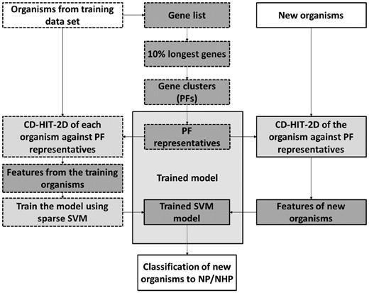
Classification workflow. Training steps are outlined in dashes, and prediction steps are outlined continuous lines. Input and output cells are colored white. Dark gray cells represent learning processes
2.2.1 Extracting features
We used CD-HIT (Li and Godzik, 2006) to construct protein clusters for use as possible classification features. CD-HIT was used for this purpose also in previous work (Cosentino et al., 2013). CD-HIT is a greedy incremental sequence clustering algorithm. Its basic algorithm sorts the input sequences according to their length and processes them sequentially from the longest to the shortest. Each protein is classified by CD-HIT either as redundant (i.e. similar to an existing representative) or as a new representative, which defines a new cluster. The sequence-similarity threshold was set to 40%, as in a previous paper (Cosentino et al., 2013).
The clustering stage is the most computationally intensive stage of training. If the CD-HIT algorithm was applied as-is to our training dataset, we estimate that it would take 22 months to finish, based on a linear extrapolation from a smaller dataset. Therefore, unlike the previous work (Cosentino et al., 2013), in our implementation we use only the longest 10% of all gene sequences in the training set as input for CD-HIT. We observe that this 10% threshold allows a reduction of the clustering time by a factor of 20 that does not reduce accuracy based on tests that we performed on a smaller dataset (discussed in detail in Section 3.1).
To further improve the running time of our clustering step, we use CD-HIT’s ‘fast mode’. In this mode, a sequence is attached to the first representative to which it is similar, without comparing it to other representatives. This is contrasted with ‘accurate mode’, in which a sequence is compared to all representatives, and cluster with the most similar one. Choosing ‘fast mode’ over ‘accurate mode’ affects only the redundant proteins, which do not define their own cluster, but has no effect on the identity of clusters or their representatives. Since our method only uses PF representatives [unlike Cosentino et al. (2013), where PF members are used as well], we run CD-HIT using the ‘fast mode’ setting. This saves many sequence comparisons, without affecting the resulting features, which are the PF representatives. This yields an additional improvement of 20% in the clustering time, as detailed in Section 3.1.
To extract an individual feature vector for each organism, we use CD-HIT-2D (Li and Godzik, 2006), which is a variant of CD-HIT that compares the protein sequences of each organism to the PFs generated from the database sequences. The output indicates which PF representatives have matches in each organism. Again, we set the threshold to 40% sequence similarity. Here we use CD-HIT’s ‘accurate mode’, which selects the most similar representative for each of the organism’s proteins. This takes longer than ‘fast mode’, however this stage can easily be distributed between different computers or CPU cores, since each organism can be compared to the PFs independently of others. Using the matching made by CD-HIT, a binary feature vector is created for each organism. The feature vector includes a coordinate for each PF. The i’th coordinate is set to 1 if the organism has a protein matching the PF representative indexed by i, and 0 otherwise.
2.2.2 Generating a classification model
We train an SVM classifier with an L1-norm penalty, using the vectors representing the organisms in the training set as input. Each such training vector is provided to the training procedure with a binary label which indicates whether it is NHP or HP. See Section 2.1 for details on how we obtained these labels. We use the L1 penalty to encourage the construction of a sparse model (i.e. a model which uses fewer features). It has been shown that the L1 penalty is a good surrogate for directly minimizing the number of features in the model, a task which is computationally infeasible (Zhu et al., 2004). We implemented the training procedure using the python package Scikit-learn (Pedregosa et al., 2012).
2.2.3 Cross-validation and scoring
We tune the model’s ‘C’ parameter (see Supplementary Section I1 in the Appendix) using standard 10-fold cross-validation (Kohavi, 1995). Due to the imbalance of the data, where HP-annotated proteomes appear ∼5 times more than NHP proteomes in the dataset, measuring regular accuracy (the proportion of correct predictions out of the validation set) would result in misleading scores which might be overly optimistic for worse models. Thus, we use instead a balanced version of the F1-score. The F1-score is the harmonic mean of precision () and recall (). By definition, both of these values are measured for the positive label of the dataset; in our case, HP. A symmetric F1-score for the negative label is the harmonic mean of the negative predictive value (NPV) () and the true negative rate (). We used the unweighted mean of both of the F1-scores described above to select the ‘C’ parameter during the cross-validation. This overcomes possible biases due to the imbalance of the labels in the training set.
3 Results
We split the dataset into 10 stratified parts, each having the same HP/NHP ratio. In every model, a different part was designated the test set, and the other nine parts were designated the training set. The proteins of the training set were then clustered to create PFs as described in Section 2.2.1. Using the resulting PF features, a stratified 10-fold cross-validation was performed within the training set, to optimize the classifier’s ‘C’ parameter (see Section 2.2.3). A classifier was then fitted on the training set, using sparse-SVM with the selected ‘C’. Lastly, the classifier was evaluated on the test set, which did not participate in the training, the cross-validation or the creation of the PFs (see Supplementary Section l3 in the Appendix). Thus, performance measures on the test set are representative of the expected performance on new proteomes never seen during the training procedure.
3.1 Quantitative results
The accuracy statistics over the 10 splits into training set and test set are given in Table 1. Full results for each split are detailed in Supplementary Table S1 in the Appendix. The shortest protein used for clustering was 527 residues long, and the shortest protein used as a cluster representative was 539 residues long.
Summary of ML accuracy results with different measures
| Scoring | Mean | Std |
|---|---|---|
| F1-macro | 0.897 | 0.0045 |
| PR-AUC | 0.992 | 0.0014 |
| ROC-AUC | 0.968 | 0.0044 |
| Sensitivity | 0.966 | 0.0072 |
| Specificity | 0.835 | 0.0287 |
| MCC | 0.795 | 0.0091 |
| Scoring | Mean | Std |
|---|---|---|
| F1-macro | 0.897 | 0.0045 |
| PR-AUC | 0.992 | 0.0014 |
| ROC-AUC | 0.968 | 0.0044 |
| Sensitivity | 0.966 | 0.0072 |
| Specificity | 0.835 | 0.0287 |
| MCC | 0.795 | 0.0091 |
Note: F1-macro, sensitivity and specificity are defined in Section 2.2.3. PR-AUC is the area under the precision-recall curve, unweighted and averaged over both labels. Note that this curve for the negative label is actually the NPV (see Section 2.2.3) versus specificity curve. ROC-AUC is the area under the ROC curve. Matthews correlation coefficient (Matthews, 1975) (MCC) is a measure of the quality of a binary confusion matrix, ranging from −1 (complete disagreement between predictions and observations) and 1 (perfect prediction).
Our average Matthews correlation coefficient (MCC) is 0.795. In comparison, a lower MCC value of 0.758 was previously reported for Pathogenfinder, a classifier that was developed and trained on a smaller dataset (Cosentino et al., 2013). Although Pathogenfinder’s dataset also contained both HP and NHP bacteria, it was not limited to human-colonizing bacteria like our dataset. Instead, it included also animal-colonizing and plant-colonizing bacteria. Proteomes of such bacteria are likely less similar, proteome-wise, to HP organisms, than non-pathogenic human-colonizing bacteria. Therefore, it would be easier for a classifier to identify them as NHP, using animal-specific or plant-specific genes. Thus, our MCC score, and our accuracy results in general, are likely more relevant to the task of distinguishing HP from NHP among human-colonizing bacteria.
The dataset that we used has a ratio of 5.45 of HP and NHPs, and so the performance of our model as reported in Table 1 pertains to this ratio. In practice the data might be skewed to have more pathogens than non-pathogens or vice versa, depending on the setting. To address this issue, we also report (see Supplementary Table S1 in the Appendix) the accuracy of our model separately for pathogens and non-pathogens, using the measures of sensitivity and specificity respectively. Since the sensitivity of our model is higher than the specificity on the test data, we conclude that our model would likely be the most accurate when the ratio tends strongly towards pathogens.
To examine how many features are necessary for our model to be accurate, we plotted F1-macro scores against the number of features that are used by the model (Fig. 2). Models with less features were generated by taking the classification model that was trained for each fold, and setting to zero the weights of all the features in this model, except for the n features with the largest absolute weight in the model . The plot in Figure 2 shows the mean F1-macro score of all 10 models, and its standard deviation. There are large differences between the maximal number of features used by trained models of different folds, from as low as 1724 for fold 3 to as high as 8649 for fold 4. Indeed, the SVM ‘C’ parameter, selected by the cross-validation process, was 0.1 for fold 2 and 100 for fold 3. These differences likely result from random differences in the content of the training set of each fold. However, the overall performance of each model on their respective test set for a similar number of features is similar. It is likely that features that are present only in a small number of models, out of the 10 models generated for the 10 different folds, are not statistically significant for pathogenicity prediction, for the type of organisms in this dataset.
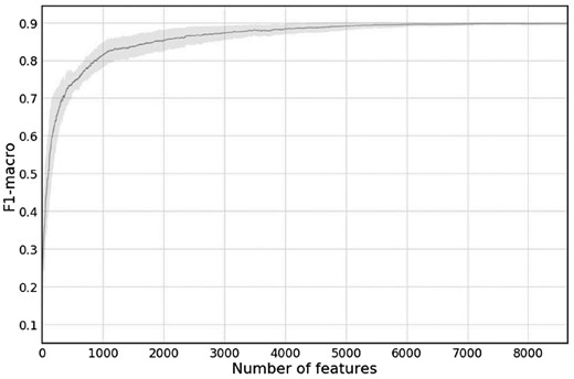
Mean F1-macro score versus number features, of each of the 10 cross-validation folds. The gray area represents the standard deviation
We trained an additional model on the entire dataset (provided in our Github directory). This model uses 9469 features. Its ‘C’ parameter was set by the cross-validation procedure to 300. This larger number of features (corresponding to this high ‘C’ value) might be due to the larger training set, which reduces the risk for overfitting, thus allowing the model to safely use more features.
3.2 Clustering using only long proteins
As described in Section 2.2.1, our training procedure rests on the hypothesis that clustering only the 10% longest genes speeds up the model training substantially, without having a significant effect on the model’s accuracy. To validate this hypothesis, we used the smaller dataset provided by Cosentino et al. (2013), on which it was feasible to compare the approaches.
In Table 2, we show the results of this comparative analysis. We compare both the model training times and their accuracy, as measured by the F1-score and by the prediction accuracy on the validation set. Here we used regular accuracy and F1-positive measures, since the validation set is relatively balanced. Our measurements show that the training time is more than 20 times faster when clustering only the 10% longest proteins of the dataset, and that this speedup does not come at the expense of accuracy or F1-score on this dataset. We observe a decline in performance only when the threshold is set to select only 2.5% of the longest genes for clustering. Moreover, we observe that the accuracy measures for different thresholds between 5 and 100% are not monotonic in the threshold, thus we propose that the differences result from statistical variation, and not from inherent deficiency of using a threshold in the range 5–100%. We selected a threshold of 10% for clustering our dataset, since this value was computationally feasible, and according to Table 2, was sufficient to preserve accuracy. Assuming a speedup of 20× holds also for our larger dataset, this means that clustering the entire set of proteins on our dataset would have taken 8 months instead of 12 days.
Comparison of computation time and accuracy of classifier when changing the threshold X for clustering the X% longest proteins
| % genes used | Computation time (days) | Accuracy | F1-score |
|---|---|---|---|
| 100 | 395 | 87.44 | 0.83 |
| 20 | 53 | 86.55 | 0.82 |
| 15 | 35 | 87.67 | 0.83 |
| 10 | 20 | 86.77 | 0.83 |
| 5 | 7 | 87.00 | 0.82 |
| 2.5 | 2 | 84.98 | 0.80 |
| % genes used | Computation time (days) | Accuracy | F1-score |
|---|---|---|---|
| 100 | 395 | 87.44 | 0.83 |
| 20 | 53 | 86.55 | 0.82 |
| 15 | 35 | 87.67 | 0.83 |
| 10 | 20 | 86.77 | 0.83 |
| 5 | 7 | 87.00 | 0.82 |
| 2.5 | 2 | 84.98 | 0.80 |
3.3 Biological results
In our final classification model, which was trained on the entire dataset, 4885 PF representatives received positive weights, linking them to an HP life-style, and 4584 representatives received negative weights, indicating that their presence in the bacterial proteomes is an indication of non-pathogenicity in humans. To gain biological insight of our results, we analyzed the 25 PF representatives that received the highest positive weights in our classification model. These PFs are expected to have a strong positive correlation between their presence in the proteomes of a bacterial strain and the involvement of this specific strain in human diseases. Supplementary Table S2 in the Appendix summarizes the characteristics of these PFs. Since we made no a priori assumptions regarding the genes that are expected to receive high positive weight, we found genes that were never reported to be related to bacterial virulence, alongside genes that are known virulence factors.
Supplementary Table S2 includes the number of HP bacteria and NHP bacteria that have each PF in their proteomes, as well as the normalized HP/NHP ratios, which corrects for the NP/NHP imbalance in the dataset. The bacterial spectrum is also presented, via the number of genera that contain the PF within their proteome. This value indicates if the PF feature is widely spread among the bacterial population, or mostly limited to a specific genus. The full list of the different genera and phyla of the organisms used in this work is available in the Supplementary Material.
Among the 25 top-scoring pathogenicity-related genes, we found genes that encode antitoxin proteins (genes 1, 9–10, 14 in the table), phage tail fiber proteins (genes 2 and 3), mobile elements (genes 8 and 20), secretion/transporter systems (genes 4 and 18) and biofilm associated proteins (genes 13 and 25). Since many virulence factors are suspected to spread by HGT, our finding that genes encoding mobile elements and phage proteins have high positive weights is not surprising. In addition, many secretion systems were previously reported to be involved in antibiotic resistance, immune system modulation and virulence mechanisms that allow pathogenic bacteria to survive within the host environment. Biofilm production allows pathogens to protect the bacterial community by forming multi-cellular structure. Antitoxin production is related to the ability of a bacterial strain to produce a potent toxin against the host cell or the commensal microflora without affecting itself.
We found several metabolic genes that received high scores (genes 6, 7, 16, 19, 21). These were involved in diverse metabolic pathways such as amino acid, nitrate and iron metabolism. While iron metabolism was previously suggested to be important for bacterial virulence, since it allows acquisition of the limited iron elements, the other metabolic pathways were not previously reported to be directly related to bacterial pathogenesis. This finding demonstrates the advantage of analyzing a combination of multiple genes that collectively can predict the nature of bacterial strains according to their proteome.
Many of the top genes on the list are uncharacterized and their function is unknown (genes 5, 10–12, 15, 17, 22–24). These genes might reveal novel virulence mechanisms that could be of great importance to understanding infectious diseases. To acquire initial information on the role of these uncharacterized genes, we examined whether any of the proteins assigned to the PF of the representative protein contain a known function. However, all proteins within the PFs of genes 10, 11, 17 and 23 were reported as hypothetical proteins with unknown functions. To examine whether they contain conserved domains of characterized proteins we analyzed them thorough NCBI Conserved Domain Search (Marchler-Bauer et al., 2017). Gene 10 in Supplementary Table S2 was found to have a conserved region, at amino acid positions 44–603, that appeared in many bacterial genes. This region was found to be 100% identical to a putative conjugal transfer protein, called TraI. This might suggest that gene 10 encodes a protein that can be translocated to other bacterial strains or is involved in the bacterial conjugation process, which allows bacteria to transfer DNA horizontally. These abilities are likely related to the pathogenicity of bacterial strains.
Gene 23 in Supplementary Table S2 was found to include a protein domain termed LXG, at positions 432–570. This protein domain is found in a group of polymorphic bacterial toxins. Such toxins are predicted to use the Type VII secretion pathway to mediate their export. We found that Gene 11 in Supplementary Table S2 contains cell-surface protein domains, suggesting it localizes on the bacterial membrane, where many virulence factors are found.
An interesting example of our model’s success is nicely demonstrated in the Acinetobacter genus. Our dataset included a relatively balanced bacterial population of this genus, with 689 HP and 627 NHP organisms. Out of these bacterial strains, 92.3% of the HP proteomes were correctly classified as HP (sensitivity) and 93.0% of the NHP proteomes were correctly classified as NHP (specificity).
At this point, we could not fully comprehend the biological correlation between the functions of the PFs that obtained the highest negative weights and the non-pathogenic bacterial life-style. It is possible that the genes required for NHP life-style are operating as multi-factorial components, and are therefore harder to correlate with specific function/activity.
3.4 Comparative results
To compare BacPaCS to the existing bacterial pathogenicity classifiers, we created an independent test set, which includes only data obtained after our model was generated. On April 27, 2018, we downloaded from the PATRIC database (Wattam et al., 2017) organisms that were added to the database after March 15, 2017 (the date in which we originally downloaded the data that was used to develop our method and to train our model). This ensured that none of these organisms was used to train our model, or the models of previous studies to which we compare. Only organisms with ‘complete’ sequencing status were downloaded, for the sake of compatibility with the PaPrBaG engine, whose training and testing format is limited to such data. This download procedure resulted in a set of 1079 organisms.
Our labeling method was then used to label these organisms. Since only 46 organisms out of the 1079 were labeled NHP by our method, we manually examined the list of organisms labeled by our method as ‘inconclusive’, and identified 10 more NHPs, using a slight modification of our labeling method (the modification is described in Section l2 in the Appendix). At this point, the list of 1079 organisms was labeled as follows: 56 NHPs, 721 HPs and 312 ‘inconclusive’. We manually validated the pathogenicity status of the 56 NHP-labeled organisms, and found that 14 of them actually had inconclusive pathogenicity status and 3 were actually pathogenic. This left us with 39 confirmed NHP organisms for our test set. To obtain confirmed HP organisms for our test set, we started with the three HPs that were found in the NHP list. We then added confirmed HP organisms to the test set by randomly selecting HP-labeled organisms from the original list of 721 organisms, and validating that they are indeed HPs. One of the randomly selected organisms was found in the manual validation to be non-pathogenic, and so it was relabeled as NHP, thus the final number of confirmed NHPs in our test set was 40. Another one of the randomly selected HP-labeled organisms was found to have an inconclusive pathogenicity status, and was removed from the test set. We stopped selecting and validating organisms from the HP list after reaching 60 confirmed HPs. This provided us with 100 bacterial genomes, out of which 40 were confirmed NHPs and 60 were confirmed HPs.
Pathogenicity labels for the organisms in the resulting set were predicted by the models of Pathogenfinder (Cosentino et al., 2013), PaPrBaG (Deneke et al., 2017) and BacPaCS. Since PaPrBaG uses raw NGS reads, WGS were downloaded, and reads were simulated using DWGSIM (https://github.com/nh13/DWGSIM), using the same definitions described in the PaPrBaG paper. For PaPrBaG predictions, we used the five models created in the 5-fold CV in the PaPrBaG paper and averaged their results. The results are given in Table 3. The list of organisms with additional details regarding the predictions by each method is given in the Supplementary Table S3 in the Appendix.
Comparative analysis results
| Tool | SEN | SPC | Classification time |
|---|---|---|---|
| BacPaCS | 0.92 | 0.48 | 18 h |
| Pathogenfinder | 0.63 | 0.28 | N/A |
| PaPrBaG | 1.00 | 0.05 | 42 min |
| Tool | SEN | SPC | Classification time |
|---|---|---|---|
| BacPaCS | 0.92 | 0.48 | 18 h |
| Pathogenfinder | 0.63 | 0.28 | N/A |
| PaPrBaG | 1.00 | 0.05 | 42 min |
BacPaCS obtained better sensitivity and specificity than Pathogenfinder, and better overall performance than PaPrBaG. The latter had very low specificity. PaPrBaG’s average running time was far shorter than BacPaCS’s. The longer running time of our model is due to the time of assigning each of the organism's proteins to its correct cluster using CD-HIT. This could easily be distributed on several machines, as explained in Section 2.2.1. Pathogenfinder’s predictions were computed on the tool’s server, since a package is not available for download. Thus, its runtime is incomparable to the rest of the tools. It should be noted that we did not test any of the models on organisms labeled as ‘inconclusive’ by our labeling method, since we do not have a reliable means of finding the true pathogenicity status of most of these organisms. Therefore, it is possible that our method would have a smaller advantage on these organisms.
4 Discussion
In this work we developed a machine-learning tool, ‘BacPaCS’, for classifying new bacterial proteomes as pathogenic to human or not. Our proposed classifier uses a large number of PFs as features, and this number greatly exceeds our available training set size, posing a risk of overfitting. To tackle this challenge, BacPaCS trains an L1-penalty SVM classifier, which naturally performs feature selection during classification. Strikingly, this results in a high-accuracy prediction tool, which is completely automated, and requires no manual configurations.
Pathogenicity classification training is highly dependent on available pathogenicity annotations. For that purpose, we created a protocol for pathogenicity annotation inference, based on phenotypes which are readily available. In the future, this protocol can be further extended and tuned for a larger database. Aside from being a prediction tool, our proposed approach can be used to reveal unknown virulence genes, as will be demonstrated in Section 3.3. In the future, we hope to determine, based on our tool, a minimal set of genes, specific for a known pathogenic genus, that can differentiate quickly and effectively between pathogenic and non-pathogenic bacterial strains. This will assist medical researchers and future clinic practitioners to develop high quality kits based on these genes.
Considering the growing size of available bacterial genome sequences, scalability is of key importance. Clustering proteins into PFs is the most computationally intensive procedure during training, making it the computational bottleneck of the training stage. Since our dataset is much larger than any previous datasets used in previous pathogenicity studies, it was crucial to speed up this process in order to make the training stage feasible. We achieved a speed up in the clustering process using two methods. First, following the approach of CD-HIT (Li and Godzik, 2006), we hypothesized that the longer protein sequences contain more sequential features (i.e. domains) than shorter protein sequences. Also, we observed that during the clustering computation, CD-HIT processes protein sequences sorted by length (longest to shortest). Therefore, it was natural to select a subset of clusters generated from the longest input sequences, and to stop the CD-HIT process once these sequences are clustered. This resulted in a significant reduction in the time needed for model training. We demonstrated in Section 3.1 that, when employing our classification approach, this does not have a significant effect on the resulting model’s accuracy. The model’s high accuracy, shown in Section 3.1, supports the validity of our hypothesis regarding the sufficiency of longer protein sequences for clustering.
Overall, the novel approach proposed in this paper yields a robust and accurate classifier to quickly differentiate HP from HNP. Although this work focused on genomics, additional data types offered by bacterial resource databases (such as transcriptomics, PPIs, three-dimensional protein structures and sequence typing data) could be considered for integration in future works.
We are confident that with the growing genetic and medical knowledge of bacterial proteomes, the accuracy of the models generated by this tool will increase.
BacPaCs requires assembled proteomes. Therefore, it currently cannot be applied to metagenomics data. However, in the future, as read lengths continue to increase, and as metagenomic binning and assembly technologies improve, the application of approaches based on protein content to metagenomics data could perhaps be reconsidered.
Although our approach was designed with pathogenicity classification in mind, it can be easily adjusted to predict phenotypes other than pathogenicity, such as antibiotic resistance.
Funding
The research of N.S. was partially supported by the Israel Science Foundation [grant number 559/15]. The research of S.S. and E.B. was partially supported by the Israel Science Foundation [grant number 555/15]. The research of M.Z.-U. and E.B. was partially supported by the Israel Science Foundation [grant number 179/14 and Grant No. 939/18].
Conflict of Interest: none declared.
References

