AssessORF: combining evolutionary conservation and proteomics to assess prokaryotic gene predictions

Abstract

Motivation

A core task of genomics is to identify the boundaries of protein coding genes, which may cover over 90% of a prokaryote's genome. Several programs are available for gene finding, yet it is currently unclear how well these programs perform and whether any offers superior accuracy. This is in part because there is no universal benchmark for gene finding and, therefore, most developers select their own benchmarking strategy.

Results

Here, we introduce AssessORF, a new approach for benchmarking prokaryotic gene predictions based on evidence from proteomics data and the evolutionary conservation of start and stop codons. We applied AssessORF to compare gene predictions offered by GenBank, GeneMarkS-2, Glimmer and Prodigal on genomes spanning the prokaryotic tree of life. Gene predictions were 88–95% in agreement with the available evidence, with Glimmer performing the worst but no clear winner. All programs were biased towards selecting start codons that were upstream of the actual start. Given these findings, there remains considerable room for improvement, especially in the detection of correct start sites.

Availability and implementation

AssessORF is available as an R package via the Bioconductor package repository.

Supplementary information

Supplementary data are available at Bioinformatics online.

1 Introduction

Gene prediction is a fundamental task of genomics, whereby protein-coding regions are delineated in a genome. Several programs have been developed for finding genes, but the extent to which any of these programs offers superior accuracy is currently unclear. This is in part because there is no universal benchmark for gene predictions. The popular gene calling programs Prodigal (Hyatt et al., 2010) and Glimmer (Delcher et al., 2007) both relied on NCBI’s GenBank annotations (Benson et al., 2017) and experimentally verified genes [e.g. the EcoGene set for E. coli (Zhou and Rudd, 2013)]. More recently, the developers of GenemarkS-2 used proteomics data and clusters of orthologous genes to validate predicted genes (Lomsadze et al., 2018). Each benchmarking approach has its own drawbacks, including the inability to detect when a predicted gene does not exist (i.e. false positives), neglecting cases where true genes are omitted (i.e. false negatives), a narrow breadth of organisms being tested and/or the inability to identify the actual start position of a gene. Given the immense number of prokaryotic genomes available, as well as the wide diversity of genome architectures used by prokaryotes, it is of considerable interest to determine the extent to which any given program outperforms others in correctly predicting prokaryotic genes.

Protein-coding genes are typically identified by their codon usage pattern, wherein certain codons appear far more frequently than they do in non-coding regions of the genome. The first well-known programs for prokaryotic gene prediction, Glimmer (Delcher et al., 1999; Salzberg et al., 1998) and GeneMark (Lukashin and Borodovsky, 1998), pioneered the use of Markov models to identify coding regions. Start codons are particularly difficult to pinpoint because multiple candidate start codons may exist near the 5'-end of a gene. For this reason, gene callers have traditionally relied on the presence of a Shine-Dalgarno sequence upstream of the start codon, although many genes do not conform to this conventional organization (Nakagawa et al., 2017). A recent update of GeneMark, GeneMarkS-2, attempts to identify genes with atypical organization (Lomsadze et al., 2018). Another well-known gene caller, Prodigal, uses multiple rounds of dynamic programming to select genes and learn their upstream motifs (Hyatt et al., 2010). Despite the differences in approaches, all programs run ab initio and learn the necessary features of a strain’s genes from the provided genomic sequence. Another source of gene boundaries is the GenBank database, which stores information about nucleotide sequences for thousands of species (Benson et al., 2017). GenBank annotations are derived from a combination of user submissions and the results of automated pipelines such as NCBI’s Prokaryotic Genome Annotation Pipeline (PGAP). PGAP uses a combination of alignment-based and ab initio methods to predict protein-coding genes, RNA genes, prophages and other regions (Tatusova et al., 2016). For protein-coding genes, PGAP first compares the proteins encoded by all of a genome’s open reading frames (ORFs) to reference protein libraries to predict genes via protein homology. PGAP then uses GeneMarkS+ (Besemer et al., 2001) to make predictions for genomic regions without protein homology.

Notably, existing gene finding programs vary by several percent in the number of genes that they identify, indicating that there remains considerable disagreement in gene predictions. Prokaryotic gene calling remains an unsolved problem for a variety of reasons. First, there are often many candidate start sites for a gene in the same ORF. This results in different programs frequently choosing conflicting start sites for the same gene, which may cause errors in downstream applications. Second, prokaryotic genes sometimes start at non-canonical codons (i.e. other than ATG, GTG and TTG) that few programs consider during the prediction process (Hecht et al., 2017). Third, despite the discovery of many short genes (i.e. <90 nucleotides) (Hücker et al., 2017; Mat-Sharani and Firdaus-Raih, 2019; Weaver et al., 2019), most gene prediction programs ignore short ORFs because of their ubiquity in the genome and lack of strong signals that allow for successful identification (Miravet-Verde et al., 2019; Storz et al., 2014). The extent to which gene finding programs fail to meet these challenges is currently unknown because existing benchmarking strategies largely focus on detecting true positives—that is, verifying the existence of predicted genes.

A variety of approaches have been used for benchmarking gene prediction algorithms. Proteomics data is considered a gold standard because genes are directly verified by their protein product (Wright et al., 2009). However, data from standard proteomics experiments typically only cover a minority of predicted genes and do not denote the exact start site of genes. In this regard, N-terminal proteomics data is particularly useful for benchmarking because it enriches for N-terminal peptides that can then be used to determine exact start sites (Willems et al., 2017). Nevertheless, N-terminal proteomics data often contains non-terminal peptides, complicating its use as a perfect benchmarking strategy (Agard and Wells, 2009). The other direct product of genes, mRNA, can be sequenced in high-throughput to confirm transcription. However, RNA-sequencing datasets lack uniformity in gene coverage, and there is no way to infer the reading frame or the exact gene start site from mRNA sequences because bacterial transcripts often include a 5' untranslated region. Ribosome profiling can be used to identify exact start sites in bacteria (Giess et al., 2017; Meydan et al., 2019), but the data is currently too rare to create a comprehensive benchmark. In contrast, the abundance of genomes for many bacterial groups makes it possible to infer start codons from their evolutionary conservation in multiple sequence alignments of syntenic regions (Dunbar et al., 2011). Start codon conservation has been applied to detect and correct mis-aligned start sites common to multiple genomes from related species (DeJesus et al., 2013; Klassen and Currie, 2013; Wall et al., 2011). A downside of this approach is that a strain may rely on a different start site than its relatives or a genomic region may be unique to a given strain, making it impossible to precisely infer start sites. Furthermore, neither of these two independent benchmarking approaches can be used to detect false positive gene predictions.

In this study, we report the development of a tool, AssessORF, for assessing prokaryotic gene predictions that combines the advantages of proteomics and evolutionary conservation into a single benchmark. In addition, AssessORF is able to detect potential false positive gene predictions through the evolutionary conservation of stop codons in related genomes. We applied AssessORF to compare four popular sources of gene predictions (Benson et al., 2017; Delcher et al., 2007; Hyatt et al., 2010; Lomsadze et al., 2018) for strains spanning the prokaryotic tree of life. Our benchmarking revealed that there remains considerable room for improvement in gene calling, with error rates averaging 5% or greater. With the exception of some short ORFs, most gene finding programs tend to correctly identify all coding regions but often select a start that is too far upstream. AssessORF is publicly available as an R package in the Bioconductor package repository (Huber et al., 2015).

2 Materials and methods

2.1 Prokaryotic strains

We sought to acquire strains for benchmarking from across the tree of life, which resulted in sampling 3 Actinobacteria, 1 Chlamydiae, 1 Crenarcheota, 1 Cyanobacteria, 8 Firmicutes and 6 Proteobacteria. Strains were selected based on the availability of proteomics data, either from in-house experiments or from literature on proteomic interrogations of microbial systems, and based on having a large number of closely related genomes available in GenBank (Benson et al., 2017). In total, we included 19 bacterial strains and one archaeal strain (Supplementary Table S1). The proteomics data for 16 of these 20 strains came from publicly available datasets while the data for the remaining four were collected as part of this study. In-house proteomics data were acquired from Acinetobacter baumannii strain ATCC 17978, Streptococcus agalactiae strain COH1, Streptococcus pyogenes strain MGAS5005 and Staphylococcus aureus strain TCH1516 (see Supplementary Methods).

2.2 Proteomics data processing

For the 16 publicly available proteomics datasets, files containing the raw mass spectrometry (MS) data from each study were downloaded from the PRIDE Archive or the MassIVe Repository, except for the Listeria dataset, where the peptide matches were downloaded directly from the PRIDE archive. Searches were performed on Proteome Discoverer using SEQUEST-HT (Eng et al., 1994) against a 6-frame translated protein database derived from each organism’s genome using a custom R script and filtered by a 5% false discovery rate (FDR) at the peptide and protein level using a reverse database strategy (Elias and Gygi, 2007; Elias et al., 2005; Peng et al., 2003). There was no strain-specific genome for Mycobacterium smegmatis so a reference genome from strain MC2 155 was used instead. Specifications for each search can be found in Supplementary Table S1. Publicly available data were searched using their originally published settings.

The in-house generated data were searched with an MS¹ tolerance of 50 ppm and MS² tolerance of 0.6 Da. Semi-tryptic digestion with a maximum of two-missed cleavages was specified. Modifications included variable oxidation of methionine, static modifications of carbamidomethylation of cysteine, and tandem mass tag labels on lysine residues and N-termini. Proteomics data generated in-house were uploaded to PRIDE through MassIVE (PXD012539—A.baumannii; PXD012567—S.agalactiae; PXD012568—S.pyogenes; PXD012538—S.aureus). Following each search, the resultant peptide spectral match (PSM) data were manually filtered to remove peptides lacking ‘High’ confidence or with ‘Rejected’ PSM ambiguity status. A database of unique peptide sequences was compiled for each set of search results.

The end result of the proteomics database searches was a set of peptide sequences and their corresponding quality scores for each of the 20 selected prokaryotic strains. The number of matched peptides ranged from 6461 to 65 481, with an average of 21 164 matched peptides per strain. Before aligning the peptide sequences to the corresponding strain’s genome, the lowest scoring 5% (i.e. equivalent to the FDR) of peptide hits were discarded to mitigate the effects of false positive peptide identifications. The remaining peptide hits were then mapped back to the focal genome (i.e. the genome of the strain of interest). Each hit was required to unambiguously map to exactly one location in the genome and was skipped otherwise.

If the sequence of a hit started with a methionine, we first attempted to match the hit to the genome without the methionine before trying the whole sequence. For most prokaryotes, N-formylmethionine is used to start the translation of new proteins, regardless of which amino acid is specified by the sequence of the start codon (Giglione et al., 2004). In most cases, this N-formylmethionine is then cleaved off in N-terminal methionine excision (NME) or deformylated by peptide deformylases soon after translation (Giglione et al., 2004). However, not all proteins undergo NME, and there is a possibility that newly translated proteins will not have undergone NME, leaving methionine in some N-terminal peptides when proteins are digested and extracted in proteomics experiments. For three of the proteomics datasets (Supplementary Table S1), a different set of extraction and digestion steps were performed to enrich for N-terminal peptides. For these three datasets, we compared the results of our standard benchmarking approach to that of treating the peptides specifically as N-terminal by requiring that the start boundaries of gene predictions be within one codon of the most upstream protein match in an ORF.

2.3 Genome alignment and evolutionary conservation

To measure evolutionary conservation of each codon position, it was first necessary to collect genomes that were closely related to each genome being assessed. To this end, we acquired all (non-partial) assemblies from each taxonomic group (e.g. genus) corresponding to a focal strain (Supplementary Table S2). Only genomes within the same taxonomic group were selected to maximize the degree of syntenic overlap with the focal strain. Related genomes that were highly similar to the focal strain’s genome were filtered based on the distance between the related genome and focal genome according to the average difference in 8-mer frequencies, $D$⁠:

$$D=\frac{{\sum }_i\left|F_i-R_i\right|}{\min (\sum F,\sum R)}$$

where F is the set of frequencies for each possible 8-mer in the focal genome and R is the corresponding set in the related genome. Only related genomes with $D\ge 1-{\left(1-\mathit{minD}\right)}^8$ were retained to ensure that genomes used to identify evolutionary conservation were not extremely similar. For $\mathit{minD}$⁠, the minimum fractional distance, a value of 0.01 was used. Up to 1000 of the most distant remaining genomes were used to determine evolutionary conservation.

Closely related genomes were aligned to the focal strain’s genome using the R package DECIPHER (Wright, 2016). This process involved mapping the syntenic regions of each related genome to the focal strain’s genome using the FindSynteny function, then aligning these collinear regions using the AlignSynteny function (Wright, 2015). To avoid artifacts due to poor alignment in a region, we applied an exponential (center-point) moving average to the vector of matches (1) and mismatches (0) along each pairwise whole genome alignment, and only considered positions in the focal genome with at least 60% average nucleotide identity in the surrounding region. A value of 60% was selected because this is above the ‘twilight zone’ of lower accuracy for nucleotide alignments. The number of times a position in the focal genome mapped to a nucleotide in related genomes was defined as the coverage at that position. At each covered position, the frequency of start codons (by default ATG, GTG and TTG) in related genomes was tabulated for positions with a start codon in the focal strain’s genome, as well as stop codons (TAG, TGA and TAA) in related genomes corresponding to any position in the focal strain's genome. These two measures were defined as start codon and stop codon conservation, respectively. Therefore, for each position, conservation divided by coverage is a normalized measure of the degree of evolutionary conservation.

2.4 The AssessORF package

Our assessment approach is provided as part of the AssessORF package (v1.2) for the R programming language (R Core Team, 2019), which is distributed under the GPLv3 license in the Bioconductor package repository (Huber et al., 2015). Usage of AssessORF occurs in two steps. First, the proteomics data and/or closely related genomes are mapped to the genome of the focal strain using the MapAssessmentData function. This results in a mapping object that can be reused to assess as many gene predictions as desired, which is useful given that the mapping process can take hours for a single genome. A separate AssessORFData package (v1.2) contains the precomputed mapping objects for each of the 20 strains analyzed in this study. Second, gene predictions for a focal strain’s genome are assessed based on how much evidence there is for or against each predicted gene in the set, which requires about 30 seconds per genome. In this step, the AssessGenes function takes a set of gene predictions and a mapping object as input and outputs a results object. The results object can then be printed, queried, plotted, or compared to other results objects.

The primary objective of AssessORF is to assign predicted genes to a category based on how much evidence there is to support each gene (Fig. 1). AssessORF gathers two types of evidence, evolutionary conservation and proteomics, which can either agree or disagree, to varying degrees, with the predicted boundaries of genes. If an ORF contains a predicted gene, the gene is assigned a character string code that has the following format: ‘Y CS[_] PE[_]’, where ‘[_]’ is replaced by a symbol describing the type of agreement or disagreement. The first part, ‘Y’ (i.e. ‘yes’), indicates that this ORF contains a predicted gene. The second part, ‘CS[_]’ (i.e. conserved start/stop), describes whether the evolutionary conservation data agrees with the predicted gene. The third part, ‘PE[_]’ (i.e. protein evidence), describes whether the proteomics data agrees with the predicted gene. We assigned qualitative category labels to each combination of assignments in order to ease user interpretation (Supplementary Table S3).

Fig. 1.

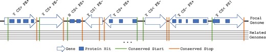
Schematic of gene categorization. AssessORF assigns each predicted gene (arrows pointing from start to stop) in a focal genome into one of 12 categories based on proteomics and evolutionary conservation evidence. Proteomics hits (blocks) allow AssessORF to classify genes into either ‘PE+’, ‘PE-’, or ‘PE!’. Aligning related genomes to the focal genome allows AssessORF to find starts that are conserved between the focal genome and related genomes and stops that are conserved in the related genomes. Conserved starts (vertical lines) enable classification of genes into either ‘CS+’, ‘CS-’, ‘CS>’, or ‘CS<’, while conserved stops in related genomes (vertical lines) reveal false positives and incorrect start sites (‘CS!’). Open reading frames with proteomics evidence but no predicted gene are classified as either ‘N CS< PE+’ or ‘N CS- PE+’ based on whether or not there is a conserved start upstream of the proteomics evidence

The CS determination uses coverage, start codon conservation and stop codon conservation. Positions in the focal genome that are not covered by at least ten genomes or 2% of the set of related genomes (by default) are marked as lacking evolutionary conservation and are not used in making a CS determination for a predicted gene (i.e. ‘CS-’). These values are large enough to ensure that estimates of conservation are founded in regions common to multiple genomes. With the remaining genome positions, AssessORF uses their degree of start codon conservation and/or their degree of stop codon conservation to assign the predicted gene to a CS category. Two parameters control whether a start codon is supported or an alternative start codon in the ORF is more likely. By default, a start codon is considered to be a strongly conserved start if it has a ratio of conservation to coverage ≥ 99%. If the ratio is <80%, the position is declared a non-conserved start. Start codons with a ratio between 80% and 99% are deemed too borderline to make a CS determination. Predicted starts are assigned to the ‘CS+’ category if they are strongly conserved (ratio ≥ 99%), have the maximum ratio value upstream of any proteomics evidence in the ORF, and there is an alternative start site somewhere in the same ORF that is not conserved (ratio < 80%). The values 99% and 80% were selected such that there is a substantial spread between potential start sites that are considered strongly conserved and not conserved. Additionally, average scores varied less than 1% when values other than 99% were employed for ratio (Supplementary Fig. S1).

To avoid the possibility of multiple start sites being classified as ‘CS+’, genes are assigned to the ‘CS-’ category when there are conserved starts other than the predicted start that have an equal or greater ratio. Conversely, if the predicted start is not conserved (ratio < 80%) and there is at least one other strongly conserved (ratio ≥ 99%) alternative start in the ORF, then the gene is assigned to ‘CS<’ or ‘CS>’ depending on whether the alternative start with the highest ratio value is upstream or downstream of the predicted start, respectively. If multiple alternative starts are tied for the maximum ratio, ‘CS<’ or ‘CS>’ is assigned based on their location, with preference given to ‘CS<’ in the case of ties. If none of the potential starts in an ORF are strongly conserved (i.e. all possible start codons have a ratio < 99%), or if all the potential starts in an ORF are conserved to some degree (i.e. have a ratio ≥ 80%), the gene is marked as lacking conserved start evidence (i.e. ‘CS-’). Importantly, all possible conserved starts must be upstream of any proteomics hits within the gene, and alternative starts must be within 200 nucleotides downstream of the previous in-frame stop and within the first half of the ORF region (by default). Over 90% of predicted start codons met these criteria, which were added to ensure that AssessORF does not give preference to conserved starts that are too close to the predicted stop. Finally, predicted genes with non-canonical starts are considered lacking CS evidence (i.e. ‘CS-’).

Stop codon conservation is used to determine whether a gene is a potential false positive prediction. A gene is categorized as ‘CS!’ if at least one codon position in the first 50% of the predicted gene corresponds to stop codons in the majority (> 50%) of related genomes covering that region. As with conserved starts, all possible positions that could be associated with a conserved stop in related genomes must be upstream of any proteomics hits within the gene. If there is proteomics evidence supporting the gene, ‘CS!’ suggests that the predicted start is too far upstream. If there is no proteomics evidence supporting the gene, ‘CS!’ suggests that the gene is a potential false positive. A conservative value of 50% was selected to require an abundance of evidence against a start codon in the rare instances where ‘CS!’ was assigned to predicted genes.

The proteomics (‘PE[_]’) categorization is based on the location of the proteomics hits relative to the predicted start. If hits within the region are all downstream of the predicted start, proteomics evidence supports the predicted gene (i.e. ‘PE+’). If any of the hits overlap with or are upstream of the predicted start, proteomics evidence contradicts the predicted start (i.e. ‘PE!’). No assessment can be made (i.e. ‘PE-’) if there are no proteomics hits within an ORF. Conversely, it is also possible to have ORFs without predicted genes but with proteomics evidence (i.e. false negatives) and are assigned to either ‘N CS< PE+’ or ‘N CS- PE+’ based on whether there is at least one strongly conserved start (ratio ≥ 99%) in the ORF upstream of the proteomics evidence. In accordance with a previous study showing that single hits are insufficient for novel gene detection (Miravet-Verde et al., 2019), at least two peptide hits are required for an ORF to be designated ‘N CS[_] PE+’.

The AssessGenes function is also able to handle situations where there are multiple predicted genes within a single ORF and situations where the predicted stop is either downstream of the ORF-ending stop, upstream of the ORF-ending stop, or out-of-frame. These latter three situations arise occasionally in GenBank records because PGAP uses frameshift and ribosomal slippage prediction to modify gene boundaries. AssessGenes assigns genes involved in any of the three situations to the no evidence category (‘Y CS- PE-’). If the predicted stop (or the most downstream predicted stop in the case of multiple genes) is downstream of the stop for the ORF, AssessGenes skips downstream ORFs until either the predicted stop or the next in-frame predicted gene is reached. If there are two or more predicted starts in the same frame that share the same ORF-ending stop, i.e. nested genes, AssessGenes assigns them to the no evidence category (‘Y CS- PE-’) by default. While it is possible that such instances represent real cases of nested genes, AssessGenes cannot determine which subset of the predicted starts is supported by any existing proteomics evidence. Predicted genes that are nested in different frames are categorized normally because AssessGenes can distinguish the evidence for each gene.

Three scores are calculated from the category assignments of each predicted gene and ORFs with proteomics evidence but no predicted gene (i.e. ‘N CS< PE+’ and ‘N CS- PE+’). The proteomics score is based on proteomics data alone:

$$\mathit{proteomics}\mathrm{ }\mathit{score}=\frac{\text{PE}+}{\text{PE}+\mathrm{ }\mathit{or}\mathrm{ }\text{PE}!}$$

The conservation score is based on evolutionary conservation assignments alone:

$$\mathit{conservation}\mathrm{ }\mathit{score}=\frac{\text{CS}+}{\text{CS}+,\mathrm{ }\text{CS}!,\mathrm{ }\text{CS}<,\mathrm{ }\mathit{or}\mathrm{ }\text{CS}>}$$

Lastly, the overall score is based on both proteomics and evolutionary conservation:

$$\mathit{overall}\mathrm{ }\mathit{score}=\frac{\mathrm{“}\mathrm{Y} \text{CS}+\text{PE}+\mathrm{”}\mathrm{ }\mathit{or}\mathrm{ }\mathrm{“}\mathrm{Y} \text{CS}+\text{PE}-”\mathrm{ }\mathit{or}\mathrm{ }\mathrm{“}\mathrm{Y} \text{CS}-\text{PE}+\mathrm{”}}{\text{PE}+,\mathrm{ }\text{PE}!,\mathrm{ }\text{CS}+,\mathrm{ }\text{CS}!,\mathrm{ }\text{CS}<,\mathrm{ }\mathit{or}\mathrm{ }\text{CS}>}$$

ORFs categorized as ‘N CS[_] PE+’ are never considered correct for any score type. Specifically, ORFs categorized as ‘N CS< PE+’ are considered when calculating all three scores while ORFs categorized as ‘N CS- PE+’ are only considered when calculating proteomics score and overall score. Notably, categories that are correct for one score type may be incorrect for other score types. For example, genes categorized as ‘Y CS< PE+’ or ‘Y CS> PE+’ are considered correct for calculating the proteomics score since they are supported by proteomics evidence. However, since evolutionary conservation evidence disagrees with the predicted start for those genes, they are considered incorrect for calculating the conservation score and the overall score. Thus, in rare instances, it is possible for the overall score to be lower than both the proteomics score and the conservation score.

2.5 Assessing gene prediction programs

A mapping object was built for each of the 20 strains using their corresponding proteomics data and set of related genomes. For each strain, Prodigal (v2.6.3), Glimmer (v3.02) and GeneMarkS-2 (web-server) were run on their default settings to generate sets of predicted genes. GenBank gene annotations for each strain's genome were also downloaded, and the boundaries for genes with CDS (i.e. coding sequence) tags were combined to form GenBank’s set of predicted genes. These four sets of predicted genes for each strain were assessed against the corresponding mapping object to produce four different results objects for each strain. The 80 total results objects were then analyzed to draw conclusions about each program's performance and are provided in the AssessORFData package. Venn diagrams were created with the VennDiagram R package to compare the four sources of gene predictions (Chen and Boutros, 2011).

3 Results

3.1 Using AssessORF to assess gene predictions

Benchmarking gene predictions is particularly challenging because there is no comprehensive gold standard that can be used as a reference. Here, we built an R package, AssessORF, for using both proteomics data and evolutionary conservation of start and stop codons to assess gene predictions. Proteomics evidence is available when a protein is produced at sufficient levels for detection. Start conservation evidence is based on the anecdotal observation that multiple sequence alignments of orthologous genes often contain a ragged left boundary implying the use of multiple alternative start sites among species (Klassen and Currie, 2013). However, there typically exists one start codon position that is highly conserved across all orthologous genes, suggesting that this conserved codon position is the true start. Neither source of evidence is perfect, as proteomics data may occasionally be a false positive hit, or a true start might exist at a non-conserved position. Notwithstanding these limitations, it is feasible to assess gene predictions for the degree to which they are supported (Supplementary Table S3) and, perhaps more importantly, to compare the relative extent of evidence across gene prediction programs.

AssessORF categorizes predicted genes (Fig. 1) based on whether there is empirical evidence supporting or against each gene. Figure 2 shows an example of assessing gene predictions made by Prodigal on the genome of Acinetobacter baumannii ATCC 17978. Most predicted genes are supported by either proteomics evidence, evolutionary conservation evidence, or both. There are also many predicted genes that have no evidence and are thus omitted from scoring. Relatively few genes are in conflict with the available evidence, and very few genes appear to be missing from the set of predictions. Notably, proteomics evidence can only be used to identify missing genes and gene starts that are too far downstream, whereas evolutionary conservation evidence can identify starts that are too far up or downstream but not missing genes. Taken together, both forms of evidence provide a more complete picture of gene prediction accuracy.

Fig. 2.

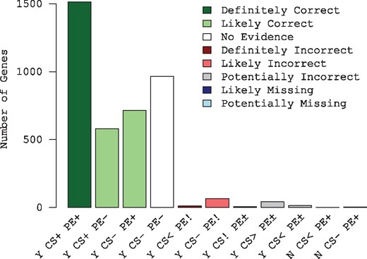
Plotting an assessment created by AssessORF. Bar plot of the number of genes in each category for the results object built from the Acinetobacter baumannii ATCC 17978 mapping object and Prodigal's predicted genes. Most genes are categorized as either ‘Y CS+ PE+’ or ‘Y CS- PE-’ meaning that they either have two forms of evidence supporting their existence or no supporting evidence, respectively

We used AssessORF to evaluate the performance of four sources of predicted genes: the programs Prodigal, GeneMarkS-2 and Glimmer, as well as the GenBank annotations for each strain. First, we compared how different sets of predicted genes generated from the four sources varied across the 20 test strains. We found that most coding regions were predicted by all four sources, as evidenced by genes sharing the same stop position (Fig. 3a). Glimmer predicted the most unique coding regions, followed by GenBank, Prodigal and GeneMarkS-2. For the 59 131 coding regions shared across all four sources, we then compared how often they shared a predicted start (Fig. 3b). In the majority of cases, all four sources picked the same start for shared genes (∼ 67% of the 59 131). However, there was greater disagreement among start positions than among stop positions, suggesting that most prediction errors are caused by picking incorrect starts. Glimmer had over twice as many unique starts (∼18%) compared to the other three sources (∼3-7%).

Fig. 3.

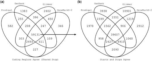
Overlap in gene predictions. (a) Venn diagram of the number of shared predicted coding regions (i.e. predicting the same stop) among Prodigal, GeneMarkS-2, GenBank and Glimmer for all 20 test strains. (b) Venn diagram of shared predicted starts for the 59 131 coding regions predicted by all four sources of gene predictions. While most starts are shared across all four, there was greater disagreement among start positions than stop positions

3.2 Comparing category assignments across sources of gene predictions

Next, we compared how category assignments varied across the four sources to determine the types of errors that are most common (Table 1). Previous studies have shown that incorrectly predicted starts are biased toward being upstream of the true gene start (Dunbar et al., 2011; Klassen and Currie, 2013). To investigate this possibility, we computed the number of genes classified as ‘CS<’ and ‘CS>’ across all strains. We disregarded protein evidence for this particular calculation because it can only provide information that a predicted start site is too far downstream. Instead, we considered conserved start evidence within N nucleotides after the upstream in-frame stop, where the predicted start was also within the first N nucleotides of the ORF. Regardless of the value of N, we found that all programs are biased towards predicting starts that are too far upstream of the conserved start, with Prodigal exhibiting the most bias and Glimmer the least (Supplementary Fig. S2). Evidence against Prodigal starts was about 2-fold to 5-fold more likely to point toward a downstream alternative start, suggesting that Prodigal systematically selects starts that are too far upstream.

Table 1.

Number of predicted genes in each category by prediction source for all 20 strains

Category	Prodigal	GeneMarkS-2	GenBank	Glimmer
Y CS+ PE+	12814	12914	12396	11067
Y CS+ PE-	4654	4628	4424	4006
Y CS- PE+	20745	20526	20327	20478
Y CS- PE-	23965	23844	23201	25998
Y CS< PE!	202	308	325	1090
Y CS- PE!	445	500	510	888
Y CS! PE+	117	92	142	161
Y CS! PE-	184	145	192	260
Y CS> PE+	261	184	315	490
Y CS> PE-	217	200	237	326
Y CS< PE+	95	141	139	395
Y CS< PE-	111	132	134	471
N CS< PE+	13	26	144	45
N CS- PE+	27	27	172	55

Short ORFs are typically omitted by gene prediction programs due to their high frequency in the genome and relatively weak coding signal. For example, Prodigal uses a minimum gene length of 90 nucleotides, but many bacterial genes shorter than this length are known (Mat-Sharani and Firdaus-Raih, 2019; Storz et al., 2014; Weaver et al., 2019). To investigate the extent to which short genes result in false negative predictions, we examined category assignments for predicted genes (across all 20 strains) by gene length (Supplementary Fig. S3). As expected, we found that shorter genes (≤ 300 nucleotides) were more frequently assigned to the no evidence category (‘Y CS- PE-’), likely because they contain fewer nucleotides for proteomics hits and conserved starts or stops. There were also more missing genes (i.e. ‘N CS- PE+’) among short ORFs than long ORFs. Glimmer predicted the most short genes and consistently had the highest error rates across all gene lengths (Supplementary Fig. S3). Furthermore, we found that GenBank missed genes more often than any other program (‘N CS< PE+’ and ‘N CS- PE+’). Nevertheless, identifiable false negative gene predictions were relatively rare for all programs (Table 1).

3.3 Comparing programs across the prokaryotic tree of life

We next sought to assess how the four sources of gene predictions varied across the twenty strains, in particular whether certain programs performed better on specific taxonomic groups. Figure 4 shows how well each program performed when considering evolutionary conservation evidence, proteomics evidence, or both types of evidence (i.e. overall score). Surprisingly, scores were generally similar across the prokaryotic tree of life, including for archaea, which are known to use distinct mechanisms for transcription initiation (Nakagawa et al., 2017). Averaging phyla equally, overall scores ranged from 0.881 (Glimmer) to 0.950 (Prodigal), suggesting that there is still considerable room for improvement in gene calling (Supplementary Table S4). On average, GenBank’s overall scores were the least correlated with the other programs across strains and displayed the greatest variability from strain-to-strain, suggesting that GenBank's performance was the least consistent. As expected, proteomics scores were higher than conservation scores because proteomics scores do not penalize for predicting a start that is too far upstream. Prodigal performed the best (15/20 strains) based on protein evidence, whereas GeneMarkS-2 performed the best (9/20 strains) based on conservation evidence. This agreed with our previous observation that Prodigal tended to predict upstream starts at a higher rate than other programs, which would increase its proteomics score by lowering the number of genes assigned to ‘PE!’ at the expense of its conservation score.

Fig. 4.

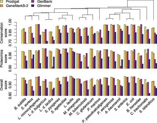
Comparison of scores across the prokaryotic tree of life. Prodigal and GeneMarkS-2 obtained the highest scores for most genomes, while GenBank's scores were more variable. Strains are sorted by their ordering in a phylogenetic tree built from the 16S ribosomal RNA gene (top)

To further compare the two top scoring programs, Prodigal and GeneMarkS-2, we explored the extent to which each program's start predictions differed for genes sharing the same stop across all 20 genomes (Fig. 5). Overall, we found that the two programs' predictions were similar in many respects, as they agreed on the start codon position in 89% of cases (55 774 shared starts out of 62 462 coding regions with shared stops) and tended to make similar types of errors. However, there were slightly more instances (793) where GeneMarkS-2’s start had conservation evidence (‘CS+’) and Prodigal’s did not (‘CS-’, ‘CS<’, or ‘CS>’) than vice versa (697). This would suggest that, for the same ORF, GeneMarkS-2 was more likely to pick the correct start than Prodigal. However, Prodigal's conservation score was slightly higher on average than that of GeneMarkS-2, although GeneMarkS-2 had the highest score for more genomes. Taken together, this suggests that variability from strain-to-strain outweighed any difference between the two programs.

Fig. 5.

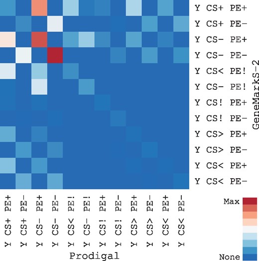
Comparison of Prodigal and GenMarkS-2 predictions. Heatmap of the set of genes where Prodigal and GeneMarkS-2 predicted the same stop but a different start in all 20 genomes. The highest values were along the diagonal where AssessORF assigned genes predicted by Prodigal and GeneMarkS-2 to the same category. There were slightly more instances where a GeneMarkS-2 start was conserved (‘CS+’) and the corresponding Prodigal start was not conserved (‘CS-’, ‘CS<’, or ‘CS>’) than vice versa

4 Discussion

In this study we developed AssessORF, a new benchmark for assessing prokaryotic gene predictions. AssessORF combines proteomics evidence with evolutionary conservation of start and stop codons to provide a more comprehensive assessment of gene callers. Applying our approach to 20 strains revealed that state of the art algorithms make gene predictions that are supported about 88 to 95% of the time (Supplementary Table S4). This leaves considerable room for improvement, particularly in the prediction of correct start sites. No program clearly outperformed all others, and all programs were biased towards choosing start sites too far upstream (Supplementary Fig. S2).

Our benchmarking approach has several limitations. First, we do not provide a set of exact start sites for each genome because the available evidence often cannot pinpoint a single start site per gene. Instead, our benchmarking approach assigns evidence to predicted genes and uses a qualitative classification scheme to represent uncertainties in gene categorizations. Ribosome profiling may offer a superior means for identifying exact start sites and provide an alternative benchmarking approach as more data of this type become available (Giess et al., 2017; Menschaert et al., 2013; Meydan et al., 2019). Second, we ignored non-canonical start sites that are neglected by all existing gene callers because of their relative rarity. Third, we did not treat N-terminal proteomics data differently because we observed the presence of many likely non-terminal peptides. For example, when we required the first peptide occurrence to align with the predicted start (or be one codon off in the case of NME), proteomics scores dropped from 0.98 with Prodigal for all three N-terminal datasets to 0.69, 0.37 and 0.29. Fourth, it is possible that multiple start codons are used for translating the same gene in some cases (Menschaert et al., 2013; Tang et al., 2016), although we ignored this potential multiplicity in our benchmarking. Such cases would result in nested genes that share the same reading frame, which are assigned to the no evidence category by AssessGenes. There were only 2 instances of nested gene pairs sharing the same reading frame among all predictions, with the 4 genes involved originating from the GenBank record for L.monocytogenes (Toledo-Arana et al., 2009). Finally, AssessORF is dependent on the quality and availability of proteomics data and closely related genomes, limiting the number of strains that can be assessed. Notwithstanding these limitations, we believe that AssessORF provides a fair depiction of the current state of the field and reveals where there is the most room for improvement in gene prediction.

The AssessORF package is particularly useful for developers of gene prediction software. Specifically, it provides tools for plotting and analyzing individual gene predictions relative to the surrounding evidence. This enables developers to focus their attention on the subset of gene predictions that are unsupported and develop ways to increase accuracy. AssessORF fills a much-needed gap in the field by providing clear measures of success, a comprehensive approach to benchmarking, a wide diversity of genomes for comparison, and the ability to expand to additional datasets in the future. Our hope is that AssessORF will accelerate improvements in gene prediction accuracy and pave the way for a new generation of gene calling algorithms.

Funding

This work was supported by the NIAID at NIH [grant number 1DP2AI145058-01]. JMW was supported by the UCSD Graduate Training Program in Cellular and Molecular Pharmacology through an institutional training grant from the NIGMS [T32 GM007752] and the UCSD Training Program in Rheumatic Diseases Research through an institutional training grant from the NIAMS [T32 AR064194]. AC was supported by the UCSD Microbial Sciences Initiative Graduate Research Fellowship and by the UCSD Graduate Training Program in Cellular and Molecular Pharmacology through an institutional training grant from the NIGMS [T32 GM007752].

Conflict of Interest: none declared.