


Abstract
Network alignment (NA) aims to find similar (conserved) regions between networks, such as cellular networks of different species. Until recently, existing methods were limited to aligning static networks. However, real-world systems, including cellular functioning, are dynamic. Hence, in our previous work, we introduced the first ever dynamic NA method, DynaMAGNA++, which improved upon the traditional static NA. However, DynaMAGNA++ does not necessarily scale well to larger networks in terms of alignment quality or runtime.
To address this, we introduce a new dynamic NA approach, DynaWAVE. We show that DynaWAVE complements DynaMAGNA++: while DynaMAGNA++ is more accurate yet slower than DynaWAVE for smaller networks, DynaWAVE is both more accurate and faster than DynaMAGNA++ for larger networks. We provide a friendly user interface and source code for DynaWAVE.
Supplementary data are available at Bioinformatics online.
1 Introduction
Network alignment (NA) aims to find a node mapping that conserves topologically or functionally similar regions between the networks, i.e. that yields high node and/or edge conservation (Vijayan et al., 2017). In computational biology, NA can predict protein function by transferring functional knowledge from well-studied to poorly-studied species between the species’ aligned cellular network regions (Faisal et al., 2015).
Until recently, existing NA methods were limited to aligning static networks. However, most real-world systems, including cellular functioning, are dynamic (i.e. they evolve over time). Static networks cannot properly model the temporal aspect of such systems, but dynamic networks can (Holme, 2015). Because of this, and as more dynamic network data are becoming available, there is a need for methods that are capable of analyzing dynamic networks, including NA methods.
So, in our previous work, we generalized static NA to dynamic NA (Vijayan et al., 2017), which (unlike static NA) explicitly exploits the temporal information from the dynamic networks being aligned. Specifically, we introduced the first method for dynamic NA, DynaMAGNA++, a generalization of a state-of-the-art static NA method MAGNA++ (Vijayan et al., 2015). MAGNA++ uses a genetic algorithm (GA) to optimize static node and edge conservation. DynaMAGNA++ inherits the GA of MAGNA++, but it optimizes measures of dynamic node and edge (event) conservation. By evaluating DynaMAGNA++ against MAGNA++ on ecological (animal proximity), cellular [protein-protein interaction (PIN)], and social (e-mail communication) networks, we showed that dynamic NA is superior to static NA.
While DynaMAGNA++ performs well, it does not necessarily scale well to larger networks, because of its GA. So, in this study, we ask whether another state-of-the-art static NA method can be generalized to its dynamic counterpart that will scale better than DynaMAGNA++. Recently, 10 static NA methods were evaluated (Meng et al., 2016), and MAGNA++, WAVE (Sun et al., 2015), and L-GRAAL (Malod-Dognin and Pržulj, 2015) produced high-quality alignments across all comparison tests. Of these methods, WAVE is the fastest. Thus, we extend WAVE from static NA to dynamic NA into a new DynaWAVE approach. Indeed, we show that DynaWAVE scales better to larger networks than DynaMAGNA++.
2 Materials and methods
First, we briefly describe the existing NA methods MAGNA++, DynaMAGNA++ and WAVE. Then, we describe our proposed dynamic NA method, DynaWAVE. All four methods are similar in the sense that they find an alignment by maximizing , where SE and SN are edge and node conservation, respectively, and β is a parameter between 0 and 1 that balances between the two conservation types. Note that SN is typically the mean of node similarities of all aligned node pairs. What the four methods differ in are the specific SE and SN measures that they optimize, as well as their optimization strategies, as follows.
MAGNA++. For this existing static NA method, SE is the S3 measure of static edge conservation (Saraph and Milenković, 2014; Vijayan et al., 2015), and SN is a static graphlet-based measure of node conservation (Kuchaiev et al., 2010; Milenković and Pržulj, 2008). MAGNA++ maximizes its objective function using a GA-based search strategy that evolves a population of alignments over a number of generations.
DynaMAGNA++. For this existing dynamic method, SE is the DS3 measure of dynamic edge conservation (Vijayan et al., 2017), and SN is a dynamic graphlet-based measure of node conservation (Hulovatyy et al., 2015). DynaMAGNA++ maximizes its objective function via MAGNA++’s GA.
WAVE. For this existing static method, SE is the weighted edge conservation (WEC) measure (see below) (Sun et al., 2015), and SN is the same static graphlet-based node conservation measure as that of MAGNA++.
WEC is a popular edge conservation measure that has since been used in other studies (Malod-Dognin and Pržulj, 2015; Mamano and Hayes, 2017). Similar to MAGNA++’s S3, WAVE’s WEC also counts the number of conserved edges, but unlike S3 which treats each conserved edge the same, WEC favors conserved edges with similar end-nodes over conserved edges with dissimilar end-nodes (for details, see Supplementary Material Section S1.1.1).
WAVE maximizes its objective function using a greedy seed-and-extend (rather than search) strategy (Supplementary Material Section S1.1).
DynaWAVE. For this proposed dynamic NA method, SE is our proposed dynamic WEC (DWEC) measure of dynamic edge (event) conservation (see below) and SN is the same dynamic graphlet-based node conservation measure as that of DynaMAGNA++.
DWEC is an extension of WEC from static NA to dynamic NA. Similar to DynaMAGNA++’s DS3, DynaWAVE’s DWEC also computes the conserved event time (CET) of the alignment where the CET of the mapping of node pair (u, v) to node pair is the amount of time during which both (u, v) and are active, and the total alignment CET is the sum of CETs across all mapped node pairs; Supplementary Material Section S1.2.1). However, unlike DS3, DWEC favors a conserved event with similar end-nodes over an equally conserved event with dissimilar end-nodes. That is, for each node pair (u, v) that is mapped to node pair , the mapping of the node pair is weighted by both the node similarities and as well as . For details, see Supplementary Material Section S1.2.1.
Similar to WAVE, DynaWAVE maximizes its objective function using a greedy seed-and-extend alignment strategy (Supplementary Material Section S1.2).
Parameters of the four methods. We set for all four methods, since WAVE, MAGNA++ and DynaMAGNA++ all use this particular parameter value in their respective papers, and since we already showed in previous work (Meng et al., 2016) that setting gives the best performance in general. Supplementary Table S1 shows our selected values for the remaining parameters of the four methods.
3 Results and discussion
We use the recently established dynamic NA evaluation framework (Vijayan et al., 2017) to compare DynaWAVE to the other three methods, as follows.
A good NA approach should produce high-quality alignments for similar networks and low-quality alignments for dissimilar networks (Guzzi and Milenković, 2017). So, we align an original dynamic real-world network (see below) to its noisy (randomized) version. We add noise to a given original network by rewiring a fraction of its events, which we refer to as the non-strict randomization model (Supplementary Material Section S2.1.1). In the main paper, we report results only for the non-strict model. Note that we analyze an additional randomization model, referred to as the strict model, which only randomizes time-stamps of the events, but not the actual events (Supplementary Material Section S2.1.2). For this model, we report results only in the supplement, due to space constraints. Nonetheless, all findings are consistent between the two models. Since with the non-strict model we only rewire events when adding noise, we know the true node mapping between the original and noisy networks. So, we can calculate the alignment quality in terms of node correctness (NC), the overlap between the given alignment and the true node mapping. We analyze three original networks: (i) the zebra proximity network (27 nodes and 779 events) (Rubenstein et al., 2015; Vijayan et al., 2017), (ii) the yeast PIN (1004 nodes and 10 403 events) (Vijayan et al., 2017) and (iii) the human aging PIN (6300 nodes and 76 666 events) (Faisal and Milenković, 2014). We vary the noise level; the higher the noise level, the more dissimilar the aligned networks. So, NC should be high at lower noise levels, and also, NC should decrease as noise increases.
When comparing dynamic NA against static NA, each of DynaWAVE and DynaMAGNA++ performs better than its static counterpart overall (Fig. 1), since the given dynamic NA method achieves higher NC at lower noise levels than its static counterpart.
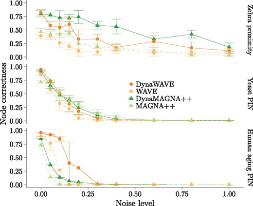
NC for DynaWAVE, WAVE, DynaMAGNA++ and MAGNA++ as a function of noise level when aligning the original network to its randomized (noisy) versions, for each of the zebra proximity network, yeast PIN and human aging PIN, for the non-strict randomization model. The error bars represent SDs over multiple runs. For each network and each noise level, each method was run five times, except that MAGNA++ and DynaMAGNA++ were run only once on the aging PIN, because of their long running times on this largest network
When comparing the two dynamic approaches, we find that DynaWAVE is: (1) less accurate but faster than DynaMAGNA++ for the smallest zebra proximity network, (2) similarly accurate and yet faster than DynaMAGNA++ for the medium-size yeast PIN and (3) both more accurate and faster than DynaMAGNA++ for the largest human aging PIN (Fig. 1, Table 1 and Supplementary Figs S1–S3).
CPU time (in minutes) of DynaWAVE, WAVE, DynaMAGNA++ and MAGNA++ when aligning each of the original networks to its noisy version
| Network | DynaWAVE | WAVE | DynaMAGNA++ | MAGNA++ |
|---|---|---|---|---|
| Zebra | 0.38 | 0.36 | 11.96 | 12.53 |
| Yeast | 0.59 | 0.49 | 311.62 | 121.47 |
| Aging | 6.43 | 5.79 | 23 499.38 | 2985.11 |
| Network | DynaWAVE | WAVE | DynaMAGNA++ | MAGNA++ |
|---|---|---|---|---|
| Zebra | 0.38 | 0.36 | 11.96 | 12.53 |
| Yeast | 0.59 | 0.49 | 311.62 | 121.47 |
| Aging | 6.43 | 5.79 | 23 499.38 | 2985.11 |
Above, we have concluded that DynaWAVE is superior to DynaMAGNA++ for large network data. However, the real-world networks that we have analyzed have not just different sizes but are also of the different types. So, next, we perform a more controlled experiment: we analyze (in the same manner as above, but focusing only on the two dynamic NA methods) synthetic networks of different sizes, where the synthetic networks come from the same random graph model and are thus of the same type. To test the robustness of results to the choice of random graph model, we repeat the entire analysis for three different models used by Vijayan et al. (2017): geometric gene duplication with probability cutoff (GEO-GD) with p = 0.3, scale-free gene duplication (SF-GD) with p = 0.3 and q = 0.7, and social network evolution (SNE) with and (Supplementary Material Section S2.2). For each network model, we vary the network size from 100 nodes to 4000 nodes in smaller increments initially and larger increments later on. Note that for the given number of nodes, the number of edges, i.e. network density, is determined automatically by the model parameters. For each network model and network size, we create three network instances, and average the results over the three runs. So, the question is: for the given synthetic network model, does DynaWAVE’s superiority become more pronounced with the increase in network size, just as it does for the real-world networks? Indeed, this is exactly what we observe (Fig. 2 and Supplementary Fig. S4).
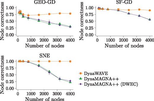
NC for DynaWAVE, DynaMAGNA++ and DynaMAGNA++ (DWEC) as a function of the number of nodes in the network when aligning the original network to itself, for synthetic networks generated using the GEO-GD, SF-GD and SNE network models. The error bars represent SDs over multiple (three) runs. Additional results, specifically when aligning the original network to its randomized (noisy) versions according to the non-strict randomization model, are shown in Supplementary Figure S4
So far, we have concluded that DynaWAVE is superior to DynaMAGNA++ for large networks, and we have verified that this holds for both real-world and synthetic networks. However, the two methods have both different objective functions and different optimization strategies (Section 2). So, next, as is typically done (Crawford et al., 2015), we aim to fairly evaluate whether it is DynaWAVE’s objective function or its optimization strategy that results in its superior performance compared to DynaMAGNA++. We test this by modifying DynaMAGNA++ so that it optimizes DynaWAVE’s objective function. We refer to this version of DynaMAGNA++ as DynaMAGNA++ (DWEC). Note that we cannot modify DynaWAVE to optimize DynaMAGNA++’s objective function, because DynaWAVE’s algorithmic design does not allow for this. By comparing DynaMAGNA++ (DWEC) against DynaMAGNA++, since the two methods share the same optimization strategy but differ in their objective functions, we can evaluate the effect of DynaWAVE’s objective function on the results. When doing so, since we find that DynaMAGNA++ (DWEC) and DynaMAGNA++ perform similarly (Fig. 2), we conclude that DynaWAVE’s objective function is not the reason for its superior performance over DynaMAGNA++. By comparing DynaWAVE against DynaMAGNA++ (DWEC), since the two methods use the same objective function but differ in their optimization strategies, we can evaluate the effect of DynaWAVE’s optimization strategy on the results. When doing so, since we find that DynaWAVE performs much better than DynaMAGNA++ (DWEC) (Fig. 2), we conclude that DynaWAVE’s optimization strategy is the reason for its superior performance over DynaMAGNA++. In summary, DynaWAVE’s superior performance compared to DynaMAGNA++, which becomes more pronounced as the network size increases, is entirely due to its optimization strategy and not its objective function.
4 Conclusion
In the recent DynaMAGNA++ study, dynamic NA was already shown to produce superior alignments compared to static NA. In this paper, we further confirm this by introducing and characterizing a novel approach for dynamic NA called DynaWAVE. Our results confirm the need for DynaWAVE as a more scalable dynamic NA approach (in terms of both accuracy and runtime) compared to DynaMAGNA++.
Funding
The Air Force Office of Scientific Research (AFOSR) [YIP FA9550-16-1-0147] and the Notre Dame Center for Research Computing.
Conflict of Interest: none declared.
References

