EPS-LASSO: test for high-dimensional regression under extreme phenotype sampling of continuous traits

Abstract

Motivation

Extreme phenotype sampling (EPS) is a broadly-used design to identify candidate genetic factors contributing to the variation of quantitative traits. By enriching the signals in extreme phenotypic samples, EPS can boost the association power compared to random sampling. Most existing statistical methods for EPS examine the genetic factors individually, despite many quantitative traits have multiple genetic factors underlying their variation. It is desirable to model the joint effects of genetic factors, which may increase the power and identify novel quantitative trait loci under EPS. The joint analysis of genetic data in high-dimensional situations requires specialized techniques, e.g. the least absolute shrinkage and selection operator (LASSO). Although there are extensive research and application related to LASSO, the statistical inference and testing for the sparse model under EPS remain unknown.

Results

We propose a novel sparse model (EPS-LASSO) with hypothesis test for high-dimensional regression under EPS based on a decorrelated score function. The comprehensive simulation shows EPS-LASSO outperforms existing methods with stable type I error and FDR control. EPS-LASSO can provide a consistent power for both low- and high-dimensional situations compared with the other methods dealing with high-dimensional situations. The power of EPS-LASSO is close to other low-dimensional methods when the causal effect sizes are small and is superior when the effects are large. Applying EPS-LASSO to a transcriptome-wide gene expression study for obesity reveals 10 significant body mass index associated genes. Our results indicate that EPS-LASSO is an effective method for EPS data analysis, which can account for correlated predictors.

Availability and implementation

The source code is available at https://github.com/xu1912/EPSLASSO.

Supplementary information

Supplementary data are available at Bioinformatics online.

1 Introduction

Extreme phenotype sampling (EPS) is a commonly used study design in genetic data analysis to identify candidate variants, genes or genomic regions that contribute to a specific disease (Cordoba et al., 2015; Zhang et al., 2014). In EPS, subjects are usually selected from the two ends of the distribution of a quantitative trait. For example, in an osteoporosis study, the top 100 and bottom 100 hip BMD subjects were recruited for gene expression analyses from a general study population (Chen et al., 2010). By enriching the presence and increasing the effect size of the causal genetic factors in the extreme phenotypic samples, EPS studies have boosted association testing power compared to studies using comparable numbers of randomly sampled subjects (Peloso et al., 2016).

With a broad application in genetic data analyses, numerous methods have been proposed to analyze data from EPS studies, such as the case–control methods. Case–control methods treat the samples with extremely high and low trait values as cases and controls, respectively. Then the standard statistical methods for group comparison (e.g. t-test) can be used to find genes with differential expression levels or frequency/proportion test to identify candidate variants with different allele frequencies (Slatkin, 1999; Wallace et al., 2006). However, the case–control methods disregard the quantitative trait values, wherein much of the genetic information may reside. Considering the inefficiency of the case–control methods, several likelihood-based methods were proposed to make full use of the available extreme phenotype data to detect associations and showed an improved power performance (Barnett et al., 2013; Huang and Lin, 2007; Lee et al., 2012).

On the other hand, most of the existing methods examine the genetic factors individually. Many phenotypes, however, are determined by multiple contributing genetic factors. Therefore, it is desirable to simultaneously model their joint effects. The joint modeling may increase the power of current genetic studies and identify novel quantitative trait loci under EPS. Considering the number (e.g. p ∼ 20 000 for transcriptomic gene expression analysis) of factors is often much greater (≫) than the study sample size (e.g. n ∼ 1000 or less), the standard linear model would not be appropriate for the joint modeling due to the rank deficiency of the design matrix. An alternative solution is to apply a penalized regression method. For instance, the least absolute shrinkage and selection operator (LASSO) can deal with the high-dimensional situations (p ≫ n) by forcing certain regression coefficients to be zero (Tibshirani, 1996). LASSO and its extensions have been increasingly employed for various genetic data analyses, such as the differential gene expression analysis (Wu, 2005, 2006), genome-wide association analysis (GWAS) (Wu et al., 2009), sequence association studies of admixed individuals (Cao et al., 2014, 2016), gene-based LASSO and group LASSO for the rare variant analysis (Larson and Schaid, 2014).

After LASSO was proposed in 1996, the statistical inference of LASSO has been broadly studied. Various algorithms were proposed to solve LASSO, including LARS (Efron et al., 2004), GLMNET (Friedman et al., 2010), SLEP (Liu et al., 2009). Procedures considering noise level were also investigated, such as the Scaled (Sun and Zhang, 2012) and Square-root (Belloni et al., 2011) LASSO. Despite that the limiting distribution of the LASSO estimator has been studied since 2000 (Fu and Knight, 2000), it was only until recently that the hypothesis testing and/or confidence intervals for LASSO were well shaped under different conditions (Bühlmann et al., 2014; Lockhart et al., 2014). Several studies proposed a debiased method for the hypothesis testing for the sparse linear or generalized linear model with Gaussian or non-Gaussian noise (Javanmard and Montanari, 2014a,b; van de Geer et al., 2014; Zhang and Zhang, 2014). Ning and Liu proposed a general testing framework based on a decorrelated score function approach and applied it to the linear regression, Gaussian graphical model and additive hazards model (Fang et al., 2016; Ning and Liu, 2017). In spite of these advancements, the statistical inference and testing for the sparse regression model under EPS remain unknown.

In view of the challenges in high-dimensional EPS genetic data analysis and lack of research for LASSO under EPS, we propose a novel sparse regression model (EPS-LASSO) using the penalized maximum likelihood for EPS. Thereafter, a hypothesis test based on a decorrelated score function for high-dimensional regression is developed to examine the significance of the associations from EPS-LASSO. We show our approach can yield stable type I error and FDR control compared to existing EPS methods through an extensive simulation study. EPS-LASSO can provide a consistent power for both low- and high-dimensional situations compared with other methods dealing with high-dimension situations. The power of EPS-LASSO is close to other low-dimensional methods under small effect sizes of causal factors and is superior when the causal effects are large. As a demonstration and also as a comparison with existing methods for extreme sampling, we apply EPS-LASSO to a transcriptome-wide gene expression study for obesity and reveal 6 significant BMI associated genes supported by previous studies and 4 novel candidate genes worth further investigation.

The rest of the paper is organized as follows. In Section 2, we present the high-dimensional regression model and an efficient algorithm to obtain the penalized estimation of parameters under EPS. The hypothesis test and its implementation are introduced in Section 2 as well. Section 3 presents the result of a simulation study to evaluate the performance of EPS-LASSO compared with other EPS methods. In addition, the result of an obesity associated gene expression analysis using real data is presented. Section 4 deliberates the limitations and areas for future studies.

2 Materials and methods

2.1 Sparse regression for EPS

Provided a dataset of $n$ independent and identically distributed pairs $\left({\mathit{x}}_{\mathit{i}},{\mathit{y}}_{\mathit{i}}\right), i=1, 2, \dots , n$⁠, we have the linear model:

$$y_i={\mathit{x}}_{\mathit{i}}^{\mathbf{\prime }}\mathit{\beta }+{\epsilon }_i,$$

(1)

where ${\mathit{x}}_{\mathit{i}}={({\mathit{x}}_{\mathit{i}1},{\mathit{x}}_{\mathit{i}2},\dots ,{\mathit{x}}_{\mathit{i}\mathit{p}})}^{\mathit{T}}$ is the set of the $p$ predictor variables; $y_i$ is the response variable for the subject $i$ and is centered to simplify the model by removing the intercept; $\mathit{\beta }={({\mathit{\beta }}_1,{\mathit{\beta }}_2,\dots ,{\mathit{\beta }}_{\mathit{p}})}^{\mathit{T}}$ is the vector of regression coefficients for the predictors; and ${\epsilon }_i$ represents the random noise. Under random sampling, it is assumed that ${\epsilon }_i\sim N(0,{\sigma }^2)$⁠, then $y_i|{\mathit{x}}_i\sim N({\mathit{x}}_{\mathit{i}}^{\mathit{\text{'}}}\mathit{\beta },{\sigma }^2)$⁠. Under EPS, the same regression model (1) can be fitted. However, the noise and phenotypic value are no longer normally distributed due to the extreme sampling (Fig. 1).

Fig. 1.

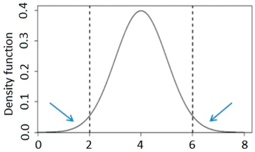
Truncated distribution under EPS. Dashed lines indicate the truncated points and the tails beyond are kept for EPS

Assuming that the upper and lower thresholds for the phenotype selection are $c_1$ and $c_2$ respectively, the extreme sampling yields that $y_i$ follows a truncated normal distribution with the probability density function (PDF):

$$f\left(y_i|{\mathit{x}}_i,c_1,c_2\right)=\frac{\Phi ({\mathit{x}}_{\mathit{i}}^{\mathbf{\text{'}}}\mathit{\beta },{\sigma }^2)}{\mathrm{\Phi }\left(c_2,{\mathit{x}}_{\mathit{i}}^{\mathbf{\text{'}}}\mathit{\beta },{\sigma }^2\right)+1-\mathrm{\Phi }(c_1,{\mathit{x}}_{\mathit{i}}^{\mathbf{\text{'}}}\mathit{\beta },{\sigma }^2)},y_i\le c_2\mathrm{or}{y}_i\ge c_1,$$

(2)

with

$$\Phi ({\mathit{x}}_{\mathit{i}}^{\mathbf{\text{'}}}\mathit{\beta },{\sigma }^2)=\frac{1}{\sqrt{2\pi {\sigma }^2}}\mathrm{e}\mathrm{x}\mathrm{p}[-\frac{({y_i-{\mathit{x}}_{\mathit{i}}^{\mathbf{\text{'}}}\mathit{\beta })}^2}{2{\sigma }^2}],$$

$$\mathrm{\Phi }(c,{\mathit{x}}_{\mathit{i}}^{\mathbf{\text{'}}}\mathit{\beta },{\sigma }^2)={\int }_{-\mathrm{\infty }}^c\frac{1}{\sqrt{2\pi {\sigma }^2}}\mathrm{e}\mathrm{x}\mathrm{p}[-\frac{({y_i-{\mathit{x}}_{\mathit{i}}^{\mathbf{\text{'}}}\mathit{\beta })}^2}{2{\sigma }^2}].$$

The log-likelihood function is:

$$\log L(\mathit{\beta },\sigma |\mathit{X})=-\frac{n}{2}\log \left(2\pi {\sigma }^2\right)-\frac{{\sum }_i{\left(y_i-{\mathit{x}}_{\mathit{i}}^{\mathbf{\text{'}}}\mathit{\beta }\right)}^2}{2{\sigma }^2}-\sum _i\log \left[\mathrm{\Phi }\left(c_2,{\mathit{x}}_{\mathit{i}}^{\mathbf{\text{'}}}\mathit{\beta },{\sigma }^2\right)+1-\mathrm{\Phi }\left(c_1,{\mathit{x}}_{\mathit{i}}^{\mathbf{\text{'}}}\mathit{\beta },{\sigma }^2\right)\right]$$

(3)

For the low-dimensional (p < n) EPS data analysis, several methods have studied the maximum likelihood estimate (MLE) of $\mathit{\beta }$ and $\sigma$ by the Newton Raphson (N-R) procedure (Barnett et al., 2013; Huang and Lin, 2007), which fails to obtain estimates for high-dimensional data. To address this challenge, we propose a penalized MLE for EPS:

$$(\widehat{\mathit{\beta }},\widehat{\sigma })=argmin\mathrm{ }(-\log L(\mathit{\beta },\sigma |\mathit{X})+\lambda \sum _{j=1}^p\left|{\beta }_j\right|),$$

(4)

where $\lambda$ is a tuning parameter controlling the sparsity $\left(s_0\right)$ of $\mathit{\beta }$⁠. The sparsity is defined as $s_0=\frac{k}{p}$⁠, where $k$ is the number of non-zero regression coefficients.

Given $\lambda$⁠, an iterative algorithm (Algorithm 1) akin to the scaled sparse regression is used to infer $\widehat{\mathit{\beta }}$ and $\widehat{\sigma }$ by solving the optimization problem (4). The initial estimate of ${\widehat{\mathit{\beta }}}^{\left(0\right)}$ is from classical Lasso. ${\widehat{\sigma }}_{MLE}>0$ is guaranteed when ${\left(Y-X\mathit{\beta }\right)}^T\left(Y-X\mathit{\beta }\right)\ne 0$ (Supplementary Note). We use the Bayesian information criterion (BIC) (Schwarz, 1978) considering both model fit and number of estimated parameters (⁠$k_{\lambda }$⁠) to select the optimum ${\lambda }^{*}$ from a series of $\lambda$ values. The BIC is adopted because of its high power and low FDR compared to cross-validation (Stone, 1974) and other high-dimensional information criterion (Supplementary Note), which also agrees with previous studies (Chen and Chen, 2012; Wang and Zhao, 2017).

$${\lambda }^{\mathrm{*}}=argmin (-2\log L+k_{\lambda }\log n)$$

At Algorithm 1 step (iii), we take the support set of converged ${\widehat{\mathit{\beta }}}^{\left(k\right)}$ at step (ii) and on its support re-estimate $\widehat{\mathit{\beta }}$ and $\widehat{\sigma }$ through the N-R procedure. The refitted estimator is motivated by the LARS-OLS hybrid strategy (Efron et al., 2004) and numerical studies from (Ning and Liu, 2017), in which the refitted estimator leads to better finite sample performance.

Algorithm 1

Estimate of $(\widehat{\mathit{\beta }},\widehat{\sigma })$ in problem (4)

Require: Data set of $\mathrm{n}$ i.i.d. pairs $\left(x_i,y_i\right)$⁠, and tuning parameter $\lambda$

(i): Initialize at k=0:

$${\widehat{\mathit{\beta }}}^{\left(k\right)}=\mathrm{a}\mathrm{r}\mathrm{g}\mathrm{m}\mathrm{i}\mathrm{n}(\frac{{\sum }_{\mathrm{i}}{\left(y_i-{\mathit{x}}_{\mathit{i}}^{\mathit{\text{'}}}\mathit{\beta }\right)}^2}{2n}+\mathrm{\lambda }{\sum }_{j=1}^p\left|{\beta }_j\right|),$$

$${\widehat{\sigma }}^{\left(k\right)}=\mathrm{a}\mathrm{r}\mathrm{g}\mathrm{m}\mathrm{i}\mathrm{n}\left(-\log L({\widehat{\mathit{\beta }}}^{\left(\mathit{k}\right)},\sigma )\right)$$

(ii): For k=k+1 until convergence:

$${\widehat{\mathit{\beta }}}^{\left(k\right)}=\mathrm{a}\mathrm{r}\mathrm{g}\mathrm{m}\mathrm{i}\mathrm{n}(-\log L(\mathit{\beta },{\widehat{\sigma }}^{\left(k-1\right)})+\lambda {\sum }_{j=1}^p\left|{\beta }_j\right|),$$

$${\widehat{\sigma }}^{\left(k\right)}=\mathrm{a}\mathrm{r}\mathrm{g}\mathrm{m}\mathrm{i}\mathrm{n}\left(-\log L({\widehat{\mathit{\beta }}}^{\left(\mathit{k}\right)},\sigma )\right)$$

(iii): Let $\widehat{S}=\{m\in \{1,\dots ,p\}:{\widehat{\beta }}_m^{\left(k\right)}\ne 0\}$⁠, ${\widehat{S}}^c$ is the complement set

  Refit $({\widehat{\mathit{\beta }}}_{\widehat{S}}, \widehat{\sigma })\mathrm{ }=argmin\left(-\log L({\mathit{\beta }}_{\widehat{\mathit{S}}},\sigma )\right)$⁠, ${\widehat{\mathit{\beta }}}_{{\widehat{S}}^c}=0$

  Return $\widehat{\mathit{\beta }}=\left({\widehat{\mathit{\beta }}}_{\widehat{S}}, {\widehat{\mathit{\beta }}}_{{\widehat{S}}^c}\right)$⁠, $\widehat{\sigma }$

2.2 Hypothesis testing

Beyond the estimate of the regression coefficients, a hypothesis testing procedure is indispensable to control the uncertainty of the regression estimate. Different from the classical statistics under low dimension, the limiting distribution of sparse estimators is largely not available (Javanmard and Montanari, 2014a,b).

Here, we develop a test statistic for the proposed EPS sparse regression model by following Ning and Liu’s general framework for high-dimensional models (Ning and Liu, 2017). Suppose we are interested in testing the null hypothesis ${\beta }_j=0$⁠, and let ${\mathit{\beta }}_{-\mathit{j}}$ denote the other regression coefficients, ${\widehat{S}}_{{\beta }_j}={\nabla }_{{\beta }_j}L\left(\widehat{\mathit{\beta }},\widehat{\sigma }|\mathit{X}\right)$and $\widehat{\mathit{I}}=-E_{\mathit{\beta }}\left({\nabla }_{\mathit{\beta }\mathit{\beta }}^{2}L\left(\widehat{\mathit{\beta }},\widehat{\sigma }|\mathit{X}\right)\right)$ be the score function and Fisher information matrix respectively, it is well known that (Cox and Hinkley, 1979):

$$n{\widehat{S}}_{{\beta }_j}^2{\widehat{I}}_{{\beta }_j|{\mathit{\beta }}_{-j}}^{-1\mathrm{ }}\sim {\chi }_{df=1}^2,$$

where ${\widehat{I}}_{{\beta }_j|{\mathit{\beta }}_{-j}}={\widehat{I}}_{{\beta }_j{\beta }_j}-\mathit{w}{\widehat{\mathit{I}}}_{{\mathit{\beta }}_{-\mathit{j}}{\beta }_j}, \mathit{w}={\widehat{\mathit{I}}}_{{\beta }_j{\mathit{\beta }}_{-\mathit{j}}}{\widehat{\mathit{I}}}_{{\mathit{\beta }}_{-\mathit{j}}{\mathit{\beta }}_{-\mathit{j}}}^{-1}$ is evaluated at the MLE under the null hypothesis. However, Ning and Liu (2017) illustrated that the classical score statistic is not valid in the high-dimensional setting, because of the asymptotically ignorable remainder converges to some intractable limiting distribution. Instead, they proposed a revised score statistic based on a decorrelated score function for a broad class of high-dimensional generalized linear model (Ning and Liu, 2017):

$$S_{{\beta }_j}^{\mathrm{*}}={\widehat{S}}_{{\beta }_j}-{\widehat{\mathit{w}}}^T{\widehat{\mathit{S}}}_{{\mathit{\beta }}_{-\mathit{j}}},$$

(5)

where $\widehat{\mathit{w}}$ is estimated by the best sparse linear combination of ${\widehat{\mathit{S}}}_{{\mathit{\beta }}_{-\mathit{j}}}$ to approximate ${\widehat{S}}_{{\beta }_j}$⁠.

For the EPS, provided the PDF and log-likelihood function in Equations (2) and (3), we have the score function $\mathit{S}={\nabla }_{\mathit{\beta }}L\left(\mathit{\beta }|\mathit{X}\right)=\frac{{\mathit{X}}^{\mathit{\text{'}}}\mathit{Y}-{\mathit{X}}^{\mathit{\text{'}}}\mathit{X}\mathit{\beta }}{{\mathit{\sigma }}^2}-\frac{{\mathit{X}}^{\mathit{\text{'}}}\mathit{M}}{\mathit{\sigma }}$⁠, where $\mathit{M}$ is a vector of length n with

$$m_i=\frac{\Phi \left(c_2-{\mathit{x}}_{\mathit{i}}^{\mathbf{\text{'}}}\mathit{\beta },{\sigma }^2\right)-\Phi \left(c_1-{\mathit{x}}_{\mathit{i}}^{\mathbf{\text{'}}}\mathit{\beta },{\sigma }^2\right)}{\mathrm{\Phi }\left(c_2,{\mathit{x}}_{\mathit{i}}^{\mathbf{\text{'}}}\mathit{\beta },{\sigma }^2\right)+1-\mathrm{\Phi }\left(c_1,{\mathit{x}}_{\mathit{i}}^{\mathbf{\text{'}}}\mathit{\beta },{\sigma }^2\right)};$$

and the Fisher information matrix $\mathit{I}=\frac{{\mathit{X}}^{\mathit{\text{'}}}\mathit{V}\mathit{X}}{{\mathit{\sigma }}^2}$⁠, in which $\mathit{V}$ is a n-dimensional diagonal matrix with the ith diagonal element

$$v_i=1-\frac{{(c}_2-{\mathit{x}}_{\mathit{i}}^{\mathbf{\text{'}}}\mathit{\beta })\Phi \left(c_2-{\mathit{x}}_{\mathit{i}}^{\mathbf{\text{'}}}\mathit{\beta },{\sigma }^2\right)-{(c}_1-{\mathit{x}}_{\mathit{i}}^{\mathbf{\text{'}}}\mathit{\beta })\Phi \left(c_1-{\mathit{x}}_{\mathit{i}}^{\mathbf{\text{'}}}\mathit{\beta },{\sigma }^2\right)}{\left[\mathrm{\Phi }\left(c_2,{\mathit{x}}_{\mathit{i}}^{\mathbf{\text{'}}}\mathit{\beta },{\sigma }^2\right)+1-\mathrm{\Phi }\left(c_1,{\mathit{x}}_{\mathit{i}}^{\mathbf{\text{'}}}\mathit{\beta },{\sigma }^2\right)\right]\sigma }-m_i^2.$$

Then, the decorrelated score function is $S_{{\beta }_j}^{*}$ defined as (5) with the $\mathit{w}$ solved by the following Lasso type estimator for the high-dimensional setting:

$$\widehat{\mathit{w}}=argmin\frac{1}{2n}\Vert {{\widehat{S}}_{{\beta }_j}-{\mathit{w}}^T{\widehat{\mathit{S}}}_{{\mathit{\beta }}_{-\mathit{j}}}\Vert }_2^2+{\lambda }^{\mathrm{\text{'}}}\sum _{d=1}^{p-1}\left|w_d\right|,$$

where ${\lambda }^{\text{'}}$ is selected by cross validation using the R package GLMNET.

With several assumptions that are commonly made on asymptotics of LASSO type estimator (Ning and Liu, 2017; van de Geer et al., 2014; Zhao and Yu, 2006), we prove the following fact for the estimate from EPS-LASSO:

$$\sqrt{n}{\widehat{S}}_{{\beta }_j}^{\mathrm{*}}{\widehat{I}}_{{\beta }_j|{\mathit{\beta }}_{-\mathit{j}}}^{-1/2}\stackrel{\mathit{d}}{\to }N(0,1).$$

The detailed proof is shown in the Supplementary Note. Finally, given the parameter estimate of $\widehat{\mathit{\beta }}$ and $\widehat{\sigma }$ in Algorithm 1, the Algorithm 2 is implemented to test the null hypothesis that ${\beta }_j=0$⁠.

Algorithm 2

Hypothesis test of ${\beta }_j=0$

Require: $(\widehat{\mathit{\beta }},\widehat{\sigma })$ from Algorithm 1

(i): Set ${\widehat{\beta }}_j=0$ and calculate $\widehat{\mathit{S}}=\frac{{\mathit{X}}^{\mathit{\text{'}}}\mathit{Y}-{\mathit{X}}^{\mathit{\text{'}}}\mathit{X}\widehat{\mathit{\beta }}}{{\widehat{\sigma }}^2}-\frac{{\mathit{X}}^{\mathit{\text{'}}}\mathit{M}}{\widehat{\sigma }}$,$\widehat{\mathit{I}}=\frac{{\mathit{X}}^{\mathit{\text{'}}}\mathit{V}\mathit{X}}{{\widehat{\sigma }}^2}$

(ii): Solve $\widehat{\mathit{w}}=argmin\frac{1}{2n}{\Vert {\widehat{S}}_{{\beta }_j}-{\mathit{w}}^T{\widehat{\mathit{S}}}_{{\mathit{\beta }}_{-\mathit{j}}}\Vert }_2^2+{\lambda }^{\text{'}}{\sum }_{d=1}^{p-1}\left|w_d\right|$

(iii): Calculate $S_{{\beta }_j}^{*}={\widehat{S}}_{{\beta }_j}-{\widehat{\mathit{w}}}^T{\widehat{\mathit{S}}}_{{\mathit{\beta }}_{-\mathit{j}}}$,${\widehat{I}}_{{\beta }_j|{\mathit{\beta }}_{-j}}={\widehat{I}}_{{\beta }_j{\beta }_j}-\mathit{w}{\widehat{\mathit{I}}}_{{\mathit{\beta }}_{-\mathit{j}}{\beta }_j}$

 p-value$=1-{\mathrm{C}\mathrm{D}\mathrm{F}}_{{\chi }_{df=1}^2}\left(n{\widehat{S}}_{{\beta }_j}^{*2}{\widehat{I}}_{{\beta }_j|{\mathit{\beta }}_{-\mathit{j}}}^{-1 }\right)=\mathbb{P}({\chi }_{df=1}^2>n{\widehat{S}}_{{\beta }_j}^{*2}{\widehat{I}}_{{\beta }_j|{\mathit{\beta }}_{-\mathit{j}}}^{-1 })$

2.3 Simulation design

To validate the proposed sparse regression model with hypothesis testing for EPS data, we simulate several typical scenarios of subjects with extreme phenotypes and genetic predictors. We assume the extreme sampling is conducted by selecting top and bottom 20% subjects from a random sampling size of 500, which results in a sample size of 200 for EPS. The number of the predictors (p) could be 100 for low-dimensional, and 200, 400 or 800 for high-dimensional situations. For each scenario, the phenotype of the ith individual in the random sampling pool is generated by a linear model:

$$y_i=\sum _{s=1}^p{\beta }_s{G}_{is}+{\epsilon }_i,$$

where ${\epsilon }_i\sim N(0, 1)$ is the random noise; and ${\beta }_s$ is the effect size of the corresponding predictor. $G_{is}$ is the sth predictor value for the ith individual, which are generated from a multivariate normal distribution ${\mathit{G}}_{\mathit{i}}\sim \mathit{N}(0,\mathit{\Sigma })$ with the covariance matrix $\mathit{\Sigma }$⁠:

$$\text{for}j\le k,\mathrm{ }{\Sigma }_{jk}=\{\begin{array}{l}\begin{array}{cc}{\rho }^{k-j}& if\mathrm{ }k\in \{j,\mathrm{ }j+1,\mathrm{ }\dots ,\mathrm{ }j+5\}\mathrm{ }\end{array}\\ \begin{array}{ll}0\mathrm{ }& \mathrm{ }\mathrm{ }for\mathrm{ }all\mathrm{ }other\mathrm{ }\end{array}j\le k\end{array},$$

${\Sigma }_{jk}={\Sigma }_{kj}$⁠, for $j>k$⁠, and $\rho$ is chosen from (0, 0.2, 0.4).

By setting all ${\beta }_s=0$⁠, a null model is used to examine the type I error. For scenarios to examine the power and FDR, we randomly pick 10 non-correlated predictors as causal factors with same non-zero ${\beta }_s$ selected from (0.1, 0.15, 0.2, 0.25, 0.3). The type I error for those non-causal causal predictors is also summarized to compare the type I error control when correlations among non-causal and causal factors are present.

2.4 Model comparison

Using the simulated datasets, we compare our model, named EPS-LASSO, with several commonly used methods for hypothesis testing including the ordinary linear model (LM), logistic regression model (LGM), linear model based on EPS likelihood (EPS-LM) and a high-dimensional Lasso testing method assuming random sampling (SSLASSO) (Javanmard and Montanari, 2014b). LM, LGM and EPS-LM are applied to test the predictors individually. In LGM, samples at the bottom and up percentiles are treated as two groups. They are all implemented in R. We prepare the EPS-LM source code based on the R package CEPSKAT. The source code for SSLASSO is downloaded from the author’s website (https://web.stanford.edu/∼montanar/sslasso/code.html). After 500 replications, the type I error, power and FDR are assessed at original and Bonferroni corrected $\alpha =0.05$ level. The type I error is defined as the proportion of significant non-causal predictors among all the non-causal predictors. The power is defined as the proportion of significant causal predictors among all the causal predictors. The FDR is defined as the proportion of significant non-causal predictors among all the significant predictors. Additionally, the absolute bias (⁠$|\widehat{\sigma }-\sigma |$⁠) of the estimate of the noise standard deviation (SD) from EPS-LASSO is compared to those from LM, EPS-LM and Scaled Lasso, respectively.

2.5 Gene expression analysis for obesity

The real data is downloaded from a substudy of Framingham Cohort project (dbGaP: phs000363) (Mailman et al., 2007; Tryka et al., 2014), which includes a profiling of 17 621 genes for 2442 Framingham Heart Study offspring subjects using the Affymetrix Human Exon 1.0 ST Gene Chip platform. The gene expression values were normalized with quality control measures as previously reported (Joehanes et al., 2013). We pick the BMI as the interested trait, which is a major characteristic of obesity. Gender, age, drinking and smoking status are considered as potential covariates. After removing the missing value in phenotypes, 972 subjects with the highest 20% or lowest 20% of BMI are selected as the EPS sample. The Bonferroni corrected significance level of 0.05 is used to claim the significance. All the simulation and real data analyses are conducted using R packages or in-house scripts available at https://github.com/xu1912/EPSLASSO.

3 Results

3.1 Simulation evaluation

We first assessed the type I error of EPS-LASSO under various null scenarios. In Figure 2 showing the P-values in scheme of 200, 400 and 800 predictors with rho (⁠$\rho$⁠) of 0 and 0.4, points from EPS-LASSO aligned close to the diagonal line and all fell in the 95% confidence region, which indicated EPS-LASSO has well-controlled type I error rates for both low- and high-dimensional situations. Conversely, LM, EPS-LM and LGM resulted in a slightly deflated type I error for high-dimensional and high-correlation scenarios, while another high-dimensional method SSLASSO inflated the type I error in some scenarios. The full result of all scenarios was summarized in the Supplementary Note. Furthermore, we examined the type I error in the scenarios with causal predictors using the scheme of 400 predictors as an example. When the causal factors were added into the null model, EPS-LASSO still controlled the type I error in the range from 0.045 to 0.055, so did the SSLASSO (Fig. 3). On the other hand, the three low-dimensional methods LM, LGM and EPS-LM yielded inflated type I error as great as ∼0.074 with the increase of the correlation between predictors (⁠$\rho$⁠) and the magnitude of the causal effect size (⁠${\beta }_s$⁠). After multiple testing correction, the type I error of EPS-LASSO was slightly inflated for large effect size (Fig. 3). SSLASSO inflated type I error under all conditions. The type I error of LM and EPS-LM were controlled when the correlation is weak (⁠$\rho$ ≤ 0.2), while the type I error of LGM was deflated. When $\rho$ is increased to 0.4, severe inflation occurred for LM and EPS-LM. These findings suggested the potential advantage of using EPS-LASSO in practice, where the correlation among predictors and multiple causal genetic factors are present.

Fig. 2.

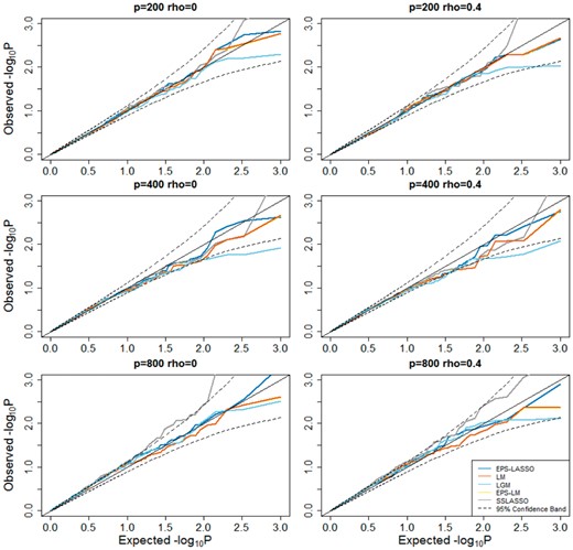
Quantile-Quantile plot for null models without causal predictors

Fig. 3.

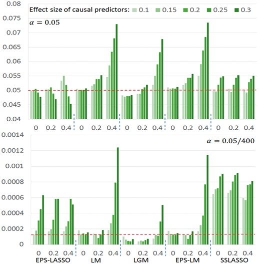
Type I error at raw (top) and Bonferroni corrected (bottom) significance level of 0.05 for scenarios with 10 causal and 390 non-causal predictors. The dashed line is the ideal level. The horizontal axis represents $\rho$ (rho). Number of predictors p = 400

We compared the power and FDR of EPS-LASSO to other methods at the Bonferroni corrected significance level of 0.05 in Figure 4. In all the scenarios, EPS-LASSO outperformed other low-dimensional methods (LM, LGM and EPS-LM) by a faster growing power with the increase of the causal effect size (Fig. 4). When the causal effect size was less than 0.2, EPS-LASSO yielded a power close to EPS-LM and LM. Then the power of EPS-LASSO exceeded others for effect size ≥0.2, while LGM resulted in the worst power due to the least information used. In addition, increasing the number of predictors led a power loss of all these methods, but EPS-LASSO was less sensitive compared with other methods in the power loss. For example, for the scenarios of ${\beta }_s=0.3$⁠, $\rho =0$⁠, the power of EPS-LASSO decreased from 86.9 to 76.5% when the number of predictors increased from 200 to 800. The relative decline of 12.0% was less than LM (13.6%), EPS-LM (14.0%) and LGM (25.4%). The FDR of low-dimensional methods were lower than EPS-LASSO for weak correlation scenarios, however, their FDR was greatly uplifted and exceeded EPS-LASSO when $\rho$ > 0.2. Due to the inflation of type I error under all conditions, we did not include the result of the other high-dimensional method SSLASSO here. But in the Supplementary Note, SSLASSO failed to gain power for low-dimensional settings with boosted FDR for high-dimensional settings. In contrast, EPS-LASSO produced a stable FDR across all scenarios and was robust to the change of effect size, number of predictors and correlation among predictors.

Fig. 4.

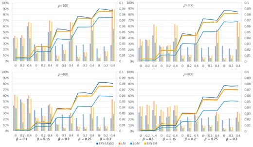
Power and FDR for scenarios with 100, 200, 400 and 800 (p) predictors. The lines aligned to the left vertical axis show the power. The histograms aligned to the right vertical axis show the FDR. The horizontal axis represents $\rho$ (rho)

Further, EPS-LASSO was superior to LM and EPS-LM with respect to the estimate of the noise SD across all the scenarios (Table 1). The absolute bias of EPS-LASSO ranged from 0.051 to 0.085 with a slightly increasing trend about the effect size. The absolute bias of EPS-LM was comparable to EPS-LASSO when the effect size was small, but increased to ∼0.372 with the increase of the effect size. The ordinary method—LM resulted in greater bias as large as ∼1.029. Another sparse model providing variance estimate—Scale-Lasso gave an even worse result, which is unstable and much greater for most cases (>100, Supplementary Table S1).

Table 1.

Absolute bias of the noise SD estimate in all scenarios

		EPS-LASSO				LM				EPS-LM
${\beta }_s$	$\rho$	p = 100	200	400	800	p = 100	200	400	800	p = 100	200	400	800
0.1	0	0.051	0.053	0.051	0.052	0.546	0.544	0.543	0.542	0.051	0.051	0.050	0.050
	0.2	0.050	0.052	0.051	0.048	0.546	0.544	0.543	0.542	0.051	0.051	0.050	0.049
	0.4	0.050	0.052	0.053	0.051	0.545	0.544	0.543	0.542	0.051	0.051	0.051	0.050
0.15	0	0.060	0.070	0.051	0.073	0.630	0.629	0.628	0.627	0.099	0.100	0.099	0.100
	0.2	0.061	0.068	0.071	0.076	0.629	0.629	0.628	0.626	0.100	0.100	0.099	0.099
	0.4	0.062	0.072	0.074	0.077	0.628	0.628	0.627	0.626	0.101	0.099	0.099	0.099
0.2	0	0.056	0.062	0.064	0.075	0.740	0.741	0.740	0.738	0.173	0.174	0.175	0.175
	0.2	0.058	0.063	0.071	0.076	0.740	0.740	0.739	0.738	0.174	0.174	0.175	0.174
	0.4	0.059	0.065	0.069	0.080	0.738	0.739	0.739	0.737	0.173	0.175	0.174	0.175
0.25	0	0.067	0.068	0.071	0.075	0.873	0.874	0.874	0.872	0.263	0.266	0.267	0.265
	0.2	0.067	0.069	0.073	0.074	0.872	0.874	0.873	0.871	0.264	0.265	0.265	0.265
	0.4	0.067	0.071	0.073	0.074	0.870	0.873	0.872	0.871	0.264	0.265	0.265	0.265
0.3	0	0.078	0.075	0.080	0.085	1.024	1.026	1.025	1.029	0.367	0.368	0.370	0.373
	0.2	0.077	0.079	0.080	0.084	1.023	1.025	1.024	1.023	0.367	0.369	0.368	0.368
	0.4	0.077	0.081	0.080	0.085	1.020	1.024	1.023	1.029	0.367	0.368	0.368	0.373

We did more simulations to illustrate the effectiveness of EPS-LASSO. First, to show the advantage of EPS-LASSO using the true distribution to infer β and σ, we compared EPS-LASSO to LASSO following the same decorrelated score test (LASSO-DST). As a result, the type I error of LASSO-DST for the high-dimensional scenarios is inflated and is close to the type I error of SSLASSO (Supplementary Note). Second, the additional analysis demonstrated the refitted estimator in Algorithm 1 can improve the power of EPS-LASSO relative to the non-refitted estimator (Supplementary Note). Third, in acknowledgement of potential issues due to re-using the same data for model selection and hypothesis testing (Chatfield, 1995; Kabaila and Giri, 2009), we examine the impact of using data multiple times in our method by simulations using 3 different datasets for tuning parameters $\lambda$⁠, $\lambda \text{'}$ and the hypothesis testing. Similar to Kabaila’s latest finding (Kabaila and Mainzer, 2017), re-use of data in our method has little effect on the performance of power and error control (Supplementary Note).

3.2 Application to obesity analysis

In order to further evaluate the performance of EPS-LASSO, we applied it and other methods to a transcriptome analysis of obesity using the EPS samples extracted from the Framingham Heart Study. From the total 17 621 assayed genes, EPS-LASSO identified 10 genes significantly (P-value < $2.84\times {10}^{-6}$⁠) associated with BMI (Table 2). Meanwhile, SSLASSO, LM, LGM and EPS-LM found 14, 576, 468 and 600 significant genes respectively. The three low dimensional methods resulted in a large number of significant findings, which may include plentiful false positive candidates and need extensive further analysis to filter out the genuine promising targets. Eight of the EPS-LASSO significant genes (MMP8, CX3CR1, UBE2J1, GCET2, ARL6IP1, TMEM111, DAAM2, TPST1) are also significant in at least one of the other methods (Table 2). Of which, MMP8, CX3CR1, UBE2J1, ARL6IP1, DAAM2 were well supported by previous studies on obesity or obesity related diseases. For example, the most significant gene MMP8 (P-value = $1.64\times {10}^{-11}$⁠), has been widely studied for its role in human obesity (Andrade et al., 2012; Belo et al., 2009). Polymorphisms in CX3CR1, UBE2J1, DAAM2 have been associated with obesity in GWAS (Do et al., 2013; Rouillard et al., 2016; Sirois-Gagnon et al., 2011). ARL6IP1 have been linked to the nonalcoholic fatty liver disease (NFLD), which is in close relation with obesity (Latorre et al., 2017). In addition, two significant genes (TMEM56 and IRS2) were detected by EPS-LASSO, but not by any of the other methods. The IRS2 gene has been reported to be a major influential gene in obesity and glucose intolerance (Lautier et al., 2003; Lin et al., 2004).

Table 2.

P-value of identifying significant genes in EPS-LASSO and other methods for the real data analysis

Gene	EPS-LASSO	EPS-LM	LM	LGM	SSLASSO	Literature
MMP8	1.64E-11	1.31E-26*	4.22E-26*	1.43E-18*	<2E-32*	Y
CX3CR1	5.01E-09	1.48E-10*	1.99E-10*	1.69E-09*	6.99E-05	Y
TMEM56	3.16E-08	7.39E-03	7.90E-03	3.38E-03	1.39E-02	N
IRS2	1.56E-07	2.68E-02	2.81E-02	5.09E-03	9.93E-03	Y
UBE2J1	2.73E-07	1.25E-18*	1.96E-18*	7.47E-18*	<2E-32*	Y
GCET2	2.87E-07	3.43E-11*	4.69E-11*	6.38E-09*	7.08E-08*	N
ARL6IP1	3.79E-07	1.49E-09*	1.99E-09*	1.20E-09*	2.84E-03	Y
TMEM111	5.88E-07	2.36E-12*	3.25E-12*	1.98E-09*	9.25E-03	N
DAAM2	1.02E-06	2.40E-13*	3.52E-13*	3.56E-10*	1.66E-06*	Y
TPST1	1.20E-06	2.04E-13*	2.92E-13*	2.52E-11*	9.32E-05	N

Note: (*) indicates significance by EPS-LM, LM, LGM and SSLASSO.

4 Discussion

In this study, we have developed a novel sparse penalized regression model with hypothesis testing for the continuous trait under extreme phenotype sampling. EPS-LASSO has stable and robust control of the type I error, especially when the predictors are correlated. In addition, EPS-LASSO can provide a persistent power for both low- and high-dimensional situations compared with the other methods dealing with high-dimensional situations. The power of EPS-LASSO is close to other low-dimensional methods under small effect sizes of causal factors and is superior to them when the causal effects are large. To demonstrate the performance of EPS-LASSO, we applied it to an EPS dataset extracted from the Framingham Heart Study. EPS-LASSO manages to identify significant BMI associated genes supported by existing studies. Overall, EPS-LASSO is a more powerful method for high-dimensional data analysis under EPS, which can account for correlated predictors.

In practice, the data type and dimension in genetic study are different by the research target and platform. Here, the straightforward application of our method in gene expression analysis shows the feasibility in analyzing several thousands of continuous genetic factors. Determined by the practical computing capability, dimension reduction is still necessary for candidate genetic factors numbered in millions, such as the genome-wide, epigenome-wide and metagenome-wide association study. A frequently used method is region-based analysis by collapsing effects or hierarchical modeling. However, the performance of the proposed method in region-based analysis needs further investigation. Other structured sparse regression methods may also be explored, like the group LASSO (Yuan and Lin, 2006).

Our method is motivated by the general theory of hypothesis test for high-dimensional models, which answers the question by dealing with the score statistic in high-dimension. There is another de-biased technique that decomposes the estimate of regression coefficients into a bias term and a normally distributed term, which facilitates the derivation of Wald statistics (Javanmard and Montanari, 2014b; van de Geer et al., 2014; Wang et al., 2016). In our method, the decorrelated score function can be regarded as an approximately unbiased estimation function for $\mathit{\beta }$ (Godambe and Kale, 1991). Also, a de-biased estimator (⁠${\stackrel{\sim }{\beta }}_j$⁠) based on the decorrelated score function can be derived by solving ${\widehat{S}}_{{\beta }_j}^{\mathrm{*}}+\left({\stackrel{\sim }{\beta }}_j-{\widehat{\beta }}_j\right){\widehat{I}}_{{\beta }_j|{\mathit{\beta }}_{-j}}=0$⁠. Given the approximate normality of ${\stackrel{\sim }{\beta }}_j$⁠, a Wald test is constructed, which is shown to be similar but slightly liberal relative to the score test regarding to the type I error, power and FDR (Supplementary Note).

In the end, we find several potential developments interesting for future exploration with EPS-LASSO. First is the dimensional reduced EPS-LASSO with the aid of initial screening. The feature screening in penalized model selection has been widely studied, including the sure screening (SS) under multiple model assumptions via marginal Pearson correlation or distance correlation (Barut et al., 2016; Fan and Lv, 2008; Fan and Song, 2010; Li et al., 2012). The SS with false selection rate control helps in power by reducing the burden of multiple testing. Given these points and a lack of study on the SS property under EPS, we consider EPS-LASSO with initial SS as an appealing direction, especially for the ultrahigh-dimensional data. Second, the FDR is not considered in EPS-LASSO. The direct application of Bonferroni correction may result in a power loss in detecting effects. Be aware of the latest application of an FDR controlled penalized regression model—SLOPE LASSO—in genetic variants under random sampling (Gossmann et al., 2015), an FDR controlled LASSO under EPS is a future direction worth pursuing.

Acknowledgements

This research was supported in part using high performance computing (HPC) resources and services provided by Technology Services at Tulane University, New Orleans, LA. The authors would like to thank the associate editor and anonymous reviewers for their valuable comments and suggestions to improve the quality of the paper.

Funding

Investigators of this work were partially supported by the grants from National Institutes of Health (NIH) [Grant Numbers: R01-AR050496-11, R01-AR057049-06, R01-AR059781-03, R01-GM109068, R01-MH104680, R01-MH104680, P20-GM109036 and U19-AG055373], National Science Foundation [Grant Number: 1539067] and Edward G. Schlieder Endowment at Tulane University.

Conflict of Interest: none declared.

Author notes

The authors wish it to be known that, in their opinion, Chao Xu and Jian Fang authors should be regarded as Joint First Authors.