Spectral clustering based on learning similarity matrix

Abstract

Motivation

Single-cell RNA-sequencing (scRNA-seq) technology can generate genome-wide expression data at the single-cell levels. One important objective in scRNA-seq analysis is to cluster cells where each cluster consists of cells belonging to the same cell type based on gene expression patterns.

Results

We introduce a novel spectral clustering framework that imposes sparse structures on a target matrix. Specifically, we utilize multiple doubly stochastic similarity matrices to learn a similarity matrix, motivated by the observation that each similarity matrix can be a different informative representation of the data. We impose a sparse structure on the target matrix followed by shrinking pairwise differences of the rows in the target matrix, motivated by the fact that the target matrix should have these structures in the ideal case. We solve the proposed non-convex problem iteratively using the ADMM algorithm and show the convergence of the algorithm. We evaluate the performance of the proposed clustering method on various simulated as well as real scRNA-seq data, and show that it can identify clusters accurately and robustly.

Availability and implementation

The algorithm is implemented in MATLAB. The source code can be downloaded at https://github.com/ishspsy/project/tree/master/MPSSC.

Supplementary information

Supplementary data are available at Bioinformatics online.

1 Introduction

Recent advances in single-cell measurements have helped scientists to better understand cellular heterogeneity (e.g. Kalisky and Quake, 2011; Pelkmans, 2012). However, single-cell datasets pose statistical and computational challenges, such as the use of single-cell data to identify groups of cells in the same functional states reflected in gene expression profiles. The identification of subgroups from single-cell data is an unsupervised classification problem, and principal component analysis (PCA), spectral clustering (von Luxburg, 2007) and k-means (Forgy, 1965) are most commonly used for subgroup identification. However, one major challenge of single cell RNA-seq (scRNA-seq) data, compared to bulk RNA-seq or gene expression microarrays, is that they have high level of noise and many missing values due to technical and sampling issues (Bacher and Kendziorski, 2016; Brennecke et al., 2013; Grün et al., 2014). The high variability in gene expression levels even among cells of the same type can confuse these existing clustering approaches (Buganim et al., 2012; Guo et al., 2010; Hashimshony et al., 2012).

Several novel clustering methods have been proposed to address these issues in scRNA-seq data analysis. For example, Xu and Su (2015) proposed a clique-based method with shared nearest neighbor similarity, which showed improved performance in identifying cell types. Sophisticated methods that involve iterative clustering have been proposed for subtype classification and the detection of relationships between the subtypes (Macosko et al., 2015; Tasic et al., 2016; Zeisel et al., 2015). Haghverdi et al. (2015) performed dimension reduction of the data by diffusion maps, which stresses continuity of cell states along putative developmental pathways. Shao and Höfer (2017) utilized a Nonnegative Matrix Factorization (NMF) technique to decompose the high-dimensional single-cell data into biologically interpretable compositions. NMF detects functional cell subgroups while simultaneously guiding the identification of biologically relevant features in the data. Wang et al. (2017) presented single-cell interpretation via multikernel learning (SIMLR), which learns a similarity measure from scRNA-seq data in order to perform dimension reduction and clustering. The critical feature of SIMLR is that it learns a similarity matrix and separates clusters by utilizing multiple kernels. These active methodology developments reflect the many challenges in unsupervised learning of biologically relevant features from scRNA-seq data.

Spectral clustering (SC) is one popular modern clustering method that uses the eigenvectors of a matrix derived from the data for clustering. SC is simple to implement, can be solved efficiently by standard linear algebra software, and often outperforms traditional clustering algorithms such as the k-means algorithm (von Luxburg, 2007). Despite of these advantages, results of SC is sensitive to choices of similarity measures, and obtaining a suitable similarity measure from scRNA-seq data requires additional efforts (Wang et al., 2017). Existing methods to improving SC performance can be categorized into two approaches (Lu et al., 2016a): (i) improve the SC clustering accuracy when a data similarity matrix is fixed; and (ii) construct an appropriate similarity matrix to improve the clustering performance. In this paper, we propose a new method that improves on both fronts. Relating to the first approach, we modify the SC framework by imposing sparse structure on the target matrix. This is motivated by the observation that this structure is essential for better clustering performance, but is not often obtained by SC when the data includes high levels of noise (Lu et al., 2016a; Wang et al., 2017). Relating to the second approach, we utilize multiple doubly stochastic affinity matrices to construct a robust similarity matrix. This can help to obtain more accurate and robust clustering results, even when the data includes many missing values and imbalanced similarities, by normalizing the similarity matrix such that all data points have equal total similarities (Lu et al., 2016b; Zass and Shashua, 2006) (e.g. Fig. 1).

Fig. 1.

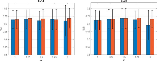
Comparisons of SC using a regular normalized affinity matrix and doubly stochastic matrix. We use the simulated data set (Simulation model 1). To construct a similarity matrix, the five kernels with σ in {1, 1.25, 1.5, 1.75, 2} are used when k = 14 and k = 20. For each pair of bars, the left and right correspond to the case of regular and doubly stochastic, respectively. The proportion of missing value is 78.6%

2 Materials and methods

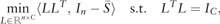
2.1 Spectral clustering

Given a set of data points $X=[x_1,\dots ,x_n]\in {ℝ}^{p\times n}$⁠, where n is the number of samples and p is the dimensionality of the data, spectral clustering (SC) uses the similarity matrix $S=\left(s_{ij}\right)\in {ℝ}^{n\times n}$⁠, where s_ij ≥ 0 represents a measure of the similarity between data points x_i and x_j. For SC to perform well, it is important to choose an appropriate similarity matrix S. Gaussian function $K(x_i,x_j)=\text{exp}\hspace{0.17em}(-{\Vert x_i-x_j\Vert }^2/(2{\sigma }^2\left)\right)$ is one of the most widely used functions to construct S (i.e. s_ij = K(x_i, x_j)), where $\Vert x_i-x_j\Vert$ is the Euclidean distance between x_i and x_j and σ controls the width of the neighborhoods. To partition data X into C clusters, SC solves the following optimization problem:

(1)

where and is a diagonal matrix with $d_{ii}={\sum }_{j=1}^n{s}_{ij}$⁠. Finally, each row of obtained L is treated as a point in ${ℝ}^C$⁠, and clustered into C groups by k-means. Note that $I_n-\overline{S}$ is called a normalized graph Laplacian (Andrew et al., 2001; von Luxburg, 2007). For detailed properties of SC, see von Luxburg (2007).

Note that in the ideal case, the orthonormal matrix $L\in {ℝ}^{n\times C}$⁠, which is the solution to (1), should have a sparse structure such that L_ij ≠ 0 iff sample i belongs to the jth cluster. Hence, LL^T should be a block diagonal matrix and thus have a sparse structure. Motivated by this observation and the fact that ${\Vert L{L}^T\Vert }_F^2=\text{tr}\left(L{L}^T\right)=C$⁠, one can consider the following regularized version of (1) to find a better U:

$$\underset{L}{\overset{}{\text{min}}}c{\Vert L{L}^T\Vert }_F^2-\langle \overline{S},L{L}^T\rangle +\lambda {\Vert L{L}^T\Vert }_1,\hspace{1em}\mathrm{s}.\mathrm{t}.\hspace{0.17em}{L}^{T}L=I_C.$$

(2)

Here adding the first term or not is mathematically equivalent, but this term provides more desired convergence properties for the proposed algorithm, which will be presented in Section 2.3.

Because (2) includes a nonlinear constraint $L^{T}L=I_C$⁠, it is not convex. To address the computational issue of the nonconvex model, we follow the idea of sparse spectral clustering (Lu et al., 2016a), which adds the relaxed convex constraints for the sparse spectral clustering:

$$\underset{P}{\overset{}{\text{min}}}c{\Vert P\Vert }_F^2-\langle \overline{S},P\rangle +\lambda {\Vert P\Vert }_1\hspace{1em}\mathrm{s}.\mathrm{t}.\hspace{0.17em}P\in \text{CH}(n,C),$$

(3)

where $\text{CH}(n,C):=\{P\in {ℝ}^{n\times n}:\hspace{0.17em}\text{tr}(P)=C,\hspace{0.17em}0\mathrm{\preccurlyeq }P\mathrm{\preccurlyeq }I\}$ and ${\Vert P\Vert }_1=\sum _{ij}^{}\left|P_{ij}\right|$⁠.

 

Remark 1 Lu et al. (2016a) also used the fact that the set CH(n, C) is a convex hull of the set $\{P=L{L}^T\in {ℝ}^{n\times n}:\hspace{0.17em}{L}^{T}L=I_C\}$⁠. It is noteworthy that (3) is strictly convex due to the additional term ${\Vert P\Vert }_F^2$⁠, so that the generalized formula (nonconvex) of (3) by using multiple similarity matrices can be computed via an iterative algorithm with convergence guarantee. See Section 2.3.1 for details.

2.2 Multiple similarity learning

Due to complexities of single cell data, relying on a single similarity may not be sufficiently informative, and we may benefit from considering multiple similarity matrices. Moreover, the performance of SC is sensitive to a single measure of similarity between data points, and there are no clear criteria to choose an optimal similarity measure. Following Wang et al. (2017), we consider multiple kernel functions to construct similarity matrices as follows: for samples i and j, 1 ≤ i ≤ j ≤ n,

$$\begin{array}{l}{K}_{\sigma ,k}(i,j)=\text{exp}\hspace{0.17em}\left(-\frac{{\Vert x_i-x_j\Vert }^2}{2{\mathrm{ϵ}}_{ij}^2}\right),\\ {\mathrm{ϵ}}_{ij}=\frac{\sigma ({\mu }_i+{\mu }_j)}{2},\hspace{0.17em}{\mu }_i=\frac{\sum _{k\in \text{KNN}\left(i\right)}^{}\Vert x_i-x_k\Vert }{k},\end{array}$$

(4)

where KNN(i) represents a set of sample indices that are the top k nearest neighbors of the sample x_i. The choices of parameters σ and k are important because they control the width of the neighborhoods and the results of SC depend on these parameters. Hence, the generalized framework using multiple kernel functions can be more adaptive to the data being analyzed than using a single kernel function. In this article, we consider σ ∈{1, 1.25,⋯, 2} and k ∈{10, 12,⋯, 30}, i.e. a total of 55 affinity matrices. More specifically, the normalized similarity matrix $G^{\left(l\right)}={\left(D^{\left(l\right)}\right)}^{-1/2}{S}^{\left(l\right)}{\left(D^{\left(l\right)}\right)}^{-1/2}$ for each l = 1,⋯, 55 is used in our analysis, where S^(l) and D^(l) are similarity and degree matrices corresponding to the lth kernel function, respectively.

2.3 Proposed method

In this section, we present the three steps of the proposed method.

Step 1: Construct a symmetric doubly stochastic similarity matrix

We use a symmetric doubly stochastic affinity matrix to construct a normalized graph Laplacian. Note that a doubly stochastic similarity matrix has been used to improve cluster analysis (Zass and Shashua, 2006; Lu et al., 2016b). This normalization is motivated by the fact that the popular affinity matrix normalization [e.g. Normalized-cuts (Shi and Malik, 2000)] is associated with a doubly-stochastic constraint (Zass and Shashua, 2006). Lu et al. (2016b) showed that t-SNE (van der Maaten and Hinton, 2008) with doubly stochastic similarity matrix input tends to provide less crowded samples in the embedding space. We observed that the performance of SC using a doubly stochastic affinity matrix for graph Laplacian is similar to or better than that using a normalized graph Laplacian (Fig. 1). We apply the Sinkhorn-Knopp iterative algorithm (SK algorithm) (Sinkhorn and Knopp, 1967) to the normalized affinity matrix G^(l) for each l and obtain a symmetric doubly stochastic matrix ${\overline{G}}^{\left(l\right)}$⁠. The SK algorithm can maintain the sparse structure of the input matrix G^(l) if it has a such structure. Note that the SK algorithm generates a sequence of matrices whose rows and columns are normalized alternately.

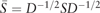
Step 2: Perform sparse spectral clustering

In the second step, we consider the optimization (3) by incorporating symmetric doubly stochastic matrices ${\overline{G}}^{\left(l\right)}$ with similarity learning:

(5)

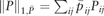where is the weighted L₁ norm of P and $\overline{P}=\left\{{\overline{p}}_{ij}\right\}$ are appropriately chosen weights. Here $W=\{w_{\ell },\hspace{0.17em}\ell =1,\dots ,N\}$ is a weight vector and λ, ρ > 0 are regularization parameters. We use ${\overline{p}}_{ij}=0$ if j ∈ KNN(i) and ${\overline{p}}_{ij}=1$ if j ∉ KNN(i), where for each data point x_i, KNN(i) is the $\tilde{k}$-nearest-neighbor using Euclidean distance.

In implementation, we use $\lambda ={10}^{-4},\hspace{0.17em}\tilde{k}=10,\hspace{0.17em}\rho =0.2$ and c = 0.1. See Supplementary Figures S2, S6–S14 for sensitivity analysis with respect to the changes of c, ρ and $\tilde{k}$⁠. Note that (5) is not jointly convex, but can be solved with iterative techniques. We use $\widehat{P}$ to denote the solution to (5).

 

Remark 2. When ρ increases to infinity, all the w_l have the same weight. Note that remains a symmetric doubly stochastic matrix. One can use different regularizations for w_l, but using the penalty yields a closed form solution of w_l in the iterative algorithm that reduces computational time.

Step 3: Shrink the pairwise difference of the target matrix

In this step, we utilize the fact that the ideal LL^T in (1) is a block diagonal matrix and thus has many equal row vectors. We consider the following optimization: for some penalty parameter μ > 0,

(6)

where the pairwise fusion penalties in (6) adaptively shrink some of $X_{j,·}-X_{k,·}$ to be zero, which is the essential idea of adaptive Lasso (Zou, 2006). Let $\widehat{X}\in {ℝ}^{n\times n}$ be the solution to (6). We obtain $\widehat{L}\in {ℝ}^{n\times C}$ by taking the first C eigenvectors corresponding to the first C largest eigenvalues of $\widehat{X}$⁠, and apply k-means to the normalized norms of $\widehat{L}$ to find the membership of the n samples. Note that (6) is also convex and can be computed using ADMM (Section A.2 of the Supplementary Material).

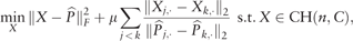
Note that Wang et al. (2017) imposed a low rank constraint on the target similarity matrix to obtain the block-diagonal structure. But a low rank matrix does not necessarily have the block-diagonal structure. We impose stronger constraints to obtain the block-diagonal structure because this structure is essential for better clustering performance. The proposed spectral clustering is different from that of Lu et al. (2016a) in the following three aspects; in the first step, we convert the normalized affinity matrix to a symmetric doubly stochastic matrix; in the second step, we use the adaptive Lasso type penalty term and include additional quadratic term ${\Vert P\Vert }_F^2$⁠; in the third step, we aim to obtain a row-wise similar target matrix using the pairwise fusion penalties to obtain the block-diagonal structure.

 

Remark 3. Instead of the two-step procedure, one can consider the following one-step optimization

(7)

which is also convex and can be computed using the ADMM algorithm. But the proposed two-step procedure is more advantageous as it uses the output matrix $\widehat{P}$ at the third stage, which adaptively penalizes the Euclidean norm of row-wise differences.

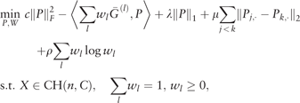
2.3.1 Algorithm

Let G(P, W) be the objective function in (5). We iteratively solve

(8)

(9)

until convergence. Note that both (8) and (9) are convex optimizations, and (8) has a closed form solution $\{w_j^{i+1},\hspace{0.17em}j=1,\dots ,N\}$⁠, where

(10)

We note that (9) can be solved via ADMM: given fixed W = Wⁱ⁺¹, we can reformulate the optimization (9) by

(11)

where the dual variables Γ_jk are the Lagrangian multipliers and η > 0 is the penalty parameter. See Section A.1 of the Supplementary Material for details. We can update P, Q and Γ iteratively. Since (9) is convex, the iterates of ADMM converge to an optimal point. Although (5) is not jointly convex, the proposed iterative Algorithm (8)–(9) enjoys convergence properties:

 

Proposition 1. Let G(P, W) be the objective function of (5). Then the iterates (Pⁱ, Wⁱ) converge to a global minimum point of G, where the objective value G(Pⁱ, Wⁱ) is monotonically decreasing.

The convergence of the proposed iterative algorithm is achieved due to the fact that G(P, W) has a unique global minimizer given one of P and W is fixed (Section B of the Supplementary Material).

2.4 Choosing the number of clusters

The proposed clustering method requires a target number of clusters. We use the following procedure to select C. First, we use a large enough number $C\prime$ as a target number and obtain $\widehat{P}$ by solving (5). Let ${\lambda }_1\ge {\lambda }_2\ge \cdots \ge {\lambda }_n\ge 0$ be the eigenvalues of $\widehat{P}$⁠. Define $C={\text{argmax}}_j\{\hspace{0.17em}{\lambda }_j-{\lambda }_{j+1}\}$⁠. We use C as a target number, i.e. we search for an index with a large eigenvalue gap of $\widehat{P}$⁠. Empirical evidence using single-cell datasets suggests that this procedure works well.

3 Simulation results

In this section, we present simulation studies to assess the performance of the proposed method. We use the following three performance metrics to evaluate the consistency between the obtained clustering and the true labels: Normalized Mutual Information (NMI) (Strehl and Ghosh, 2003), Purity and Adjusted Rand Index (ARI) (Wagner and Wagner, 2007b). NMI and Purity take on values between 0 and 1, but ARI can yield negative values. These metrics measure the concordance of two clustering labels such that higher value refers to higher concordance. For details of these metrics, see Section D of the Supplementary Material.

 

Remark 4. ARI is one of the metrics based on counting pairs of objects. Note that ARI relies on the strong assumptions on the distribution on clusterings; it assumes a generalized hypergeometric distribution as the null hypothesis, i.e. the two clusterings are drawn randomly with a fixed number of clusters and a fixed number of elements in each cluster (Wagner and Wagner, 2007a). Purity is one of the measures relying on a mapping, which is not one-to-one. This mapping may be biased towards the cluster which has the largest size (Wagner and Wagner, 2007a). NMI is based on mutual information, which has its origin in information theory and is based on the notion of entropy. Note that NMI does not suffer from the drawbacks that one can find for metrics that are based on counting pairs or mappings (Wagner and Wagner, 2007a).

In the experiments, we use two types of simulation data. We generate the first simulation model using the following four steps. In the first step, we generate C points in the 2-dimensional latent space to create a circle, each point is considered to be the center of one cluster. The n points are generated by adding independent noise to the center of the corresponding cluster. In the second step, we project the generated 2-dimensional data to a p-dimensional space, which represents gene expression data. In the third step, we simulate a noisy gene expression matrix by adding independent Gaussian noise. In the last step, we introduce a dropout event such that each entry is independently observed with a certain probability. In the second simulation model, we generate the data using Gaussian mixture model. To distinguish different cell types, it is likely that only some genes are informative, and non-informative and highly noisy genes can increase the difficulty of identifying cell types. Under this context, we use a few attributes to distinguish the clustering labels in the simulation models. For details of these simulation models, see Section E of the Supplementary Material.

In the first experiment, we compare the performances of SC by using different graph Laplacians obtained by the regular normalized affinity matrix and the doubly stochastic matrix. Figure 1 shows the average NMI values and one standard deviation of the SC with ten selected affinity matrices based on k ∈{14, 20} and σ ∈{1, 1.25, 1.5, 1.75, 2} for the two different graph Laplacians. We can see that the doubly stochastic affinity matrix based SC performs similar or better than the SC with the regular normalized affinity matrix. In addition, we see that the clustering performance varies across different kernels used to construct an affinity matrix. This illustrates the need for a new spectral clustering method that does not rely on a single similarity measure, and for this purpose we utilize multiple similarity matrices as presented in Section 2.2.

In the second experiment, we investigate the robustness of the clustering performance of the proposed clustering method with respect to the change of regularization parameters $c,\tilde{k},\lambda$ and μ. We choose c from {0.01, 0.05, 0.1, 1}, $\tilde{k}$ from {5, 10,⋯, 80} and λ and μ from {10^–5, 10^–4, 10^–3, 10^–2}. We see that the clustering results are robust with respect to the changes in these parameters, and stable clustering results could be achieved by many different combinations of $c,\tilde{k},\lambda$ and μ settings (Supplementary Fig. S2). Specifically, we observe that the performance is consistently good when c = 0.1, $\tilde{k}=10$ and λ = μ = 10^–4. Therefore, in the following applications we use these values. Note that Lu et al. (2016a) also included sensitivity analysis for λ in their modified SC formula, and proposed to use λ = 10^–4. For the sensitivity of the choice of ρ, see Supplementary Figure S2F. In implementation, we fix ρ = 0.2, which performs well for various settings. Sensitivity analysis of these parameters for the real scRNA-seq datasets (Supplementary Figs S6–S14) also shows the robustness of the proposed clustering method with respect to the changes of these parameters.

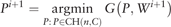
In the third experiment, to investigate the effect of the similarity learning using multiple affinity matrices, more intuitively, we show the heat map of the $\left|V{V}^T\right|={\left(\right|V_{i,·}{V}_{j,·}^T\left|\right)}_{i,j}$⁠, where $V\in {ℝ}^{n\times C}$ has orthonormal columns consisting of the C eigenvectors corresponding to the first C largest eigenvalues of $\widehat{P}$⁠. Here $\widehat{P}\in {ℝ}^{n\times n}$ is the obtained target matrix by any SC methods. In the ideal case, |V V ^T| should have the block diagonal structure. Figure 2 shows the heat map of the |V V ^T|: Figure 2A and B consider the standard SC using different similarity matrices. Figure 2C considers the proposed method without Step 3. Figure 2D uses the proposed method as in Section 2.3. For Figure 2A and B, we choose the kernel having the smallest kernel weight, 0.0022, and the largest kernel weight, 0.032 in the proposed spectral clustering used in Figure 2D. Interestingly, the structure in Figure 2B is more similar to the block diagonal structure compared with Figure 2A, which shows that the proposed method tends to give a larger weight to a kernel that provides clearer block diagonal structure. We observe that Figure 2D has a clearer block diagonal structure compared with Figure 2A, B and C, which shows that similarity learning and Step 3 help recover the true structure.

Fig. 2.

Heat maps of |VV^T| for the standard SC using a single Kernel of σ = 2 and k = 30 (A) and σ = 1 and k = 10 (B). Heat maps of |VV^T| for the proposed method without Step 3 (C) and for the proposed method (D). The data follows Simulation model 1

In the last experiment, we compare the proposed method without similarity learning (‘PSSC’) and the proposed method (‘MPSSC’), with the following four existing methods: t-SNE (van der Maaten and Hinton, 2008); SIMLR (Wang et al., 2017); Spectral clustering (‘SC’); and Sparse spectral clustering (‘SSC’) (Lu et al., 2016a). For the PSSC, we use the average similarity matrix from 55 considered kernels. For SSC, we use the regularized parameters suggested by Lu et al. (2016a). Figure 3A and B show the average NMI value with one standard deviation (error bars) for Simulation model 1. When γ = 0.01 (missing proportion is 37%), MPSSC, PSSC, SIMLR and tSNE have similar NMI values and outperform the SC and SSC. The paired sample t-test shows that the mean differences of SC, SSC and PSSC from MPSSC are significant (P-value < 0.001), but the mean differences of t-SNE and SIMLR from MPSSC are not significant (P-values= 0.08 and 0.16, respectively). When γ = 0.006 (missing proportion is 90%), MPSSC outperforms the other methods. The P-values of the other methods from MPSSC are significant (P-value < 0.002). The results of Simulation model 2 (Fig. 3C and D) show that MPSSC, PSSC and SSC have higher values than the other methods. For (C), the paired sample t-test suggests that the mean differences of SC, t-SNE and SIMLR from MPSSC are significant (P-value < 0.001), but the P-values of SSC and PSSC are 0.81 and 0.55, respectively. For (D), the P-values of SC, t-SNE and SIMLR from MPSSC are significant (P-value < 0.001), but the P-values SSC and PSSC are 0.07 and 0.44. To sum up, we observe that MPSSC and PSSC consistently have higher values, compared with other methods, which suggests that MPSSC and PSSC can identify clusters in accurately and robustly.

Fig. 3.

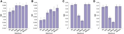
 (A) and (B): Average performance values with one standard deviation of the six clustering methods when γ = 0.01 (A) and γ = 0.006 (B). The proportions of missing values are 37% and 90% for (A) and (B), respectively. The results are based on simulating 50 datasets following Simulation model 1; C and D: Average performance values with one standard deviation of the seven clustering methods when γ = 0.6 (A) and γ = 0.1 (B). The proportions of missing values are 56 and 67% for (C) and (D), respectively. The results are based on 50 datasets simulated following Simulation model 2. See Section E of the Supplementary Material for details of the simulation models and γ

4 Applications to single-cell RNA sequence data

In this section, we apply the proposed clustering methods to single-cell RNA-Seq datasets to demonstrate their clustering performances compared with existing clustering methods. We collected nine scRNA-seq datasets representing several types of dynamic processes such as cell differentiation, cell cycle and response upon external stimulus. Each scRNA-seq data contains cells for which the labels were known a priori or validated in the respective studies. The characteristics of the nine datasets are summarized in Table 1. For detailed description of the nine scRNA-seq datasets, see Section F of the Supplementary Material.

Table 1.

Summary of the characteristics of the nine real single-cell datasets

Dataset	# cells (n)	# genes (p)	# cell types
Deng (Deng et al., 2014)	135	12548	7
Ginhoux (Schlitzer et al., 2015)	251	11834	3
Ting (Ting et al., 2014)	114	14405	5
Treutlein (Treutlein et al., 2014)	80	9352	5
Buettner (Buettner et al., 2015)	182	8989	3
Pollen (Pollen et al., 2014)	249	14805	11
Tasic (Tasic et al., 2016)	1727	5832	49
Zeisel (Zeisel et al., 2015)	3005	4412	47
Macosko (Macosko et al., 2015)	6418	12822	39

We compare the PSSC and MPSSC with the other methods using the three metrics as in Section 3. For PSSC and MPSSC, we first estimate the number of clusters using the method presented in Section 2.4. For the other methods, we use the true cluster number to obtain the clustering results. Figure 4 summarizes NMI and computational time for the six small-scale single cell datasets. In many cases, the MPSSC and PSSC have higher NMI values, which shows that they generally perform better than their competitors. This demonstrates that the proposed methods can better uncover cell-to-cell similarity and dissimilarity structures than other competitors. They also have comparable computation time with other methods. Figure 5 summarizes NMI and computation time for three larger-scale datasets. For larger-scale datasets, we have conducted the MPSSC and PSSC without the third step due to time complexity and memory issue. We observe that the proposed methods MPSSC and PSSC still have higher NMI values, while computation times are comparable to SSC and SIMLR. For Purity and ARI measures, see Supplementary Figures S4–S5.

Fig. 4.

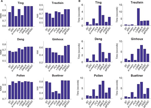
Evaluation of the eight clustering methods by NMI (A) and computational time (B) for the six small-scale datasets, implemented on an Apple MacBook Pro (2.7 GHz, 8 GB of memory) using the MATLAB 2016b

Fig. 5.

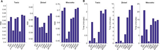
Evaluation of the eight clustering methods by NMI (A) and computational time (B) for the three large-scale datasets, implemented on the computing cluster (6 CPUs, 800 GB of memory)

Among the nine datasets, we mainly analyze the two datasets based on the clustering results. The first dataset, called the Ginhoux dataset (Schlitzer et al., 2015) in Table 1, contains the expression values of 11 834 genes for 251 dendritic cell progenitors in one of three cellular states: Monocyte and Dendritic cell Progenitors (MDPs), Common Dendritic cell Progenitors (CDPs) and Pre-Dendritic Cells (PreDCs). DC progenitors are derived from hematopoietic stem cells in the bone marrow, and transition through a plethora of cellular states before becoming fully developed DC (Schlitzer et al., 2015). The dataset contains 59 MDPs, 96 CDPs and 96 PreDCs. Although dendritic cells play an important role in the activation of the adaptive immune systems in vertebrates, several mechanisms involved in this process are controversial (Cannoodt et al., 2016; Murphy et al., 2016; Winter and Amit, 2015). Figure 6A visualizes the cells in 2-D space using MPSSC. For visualization, we utilize the obtained $\widehat{P}$ of MPSSC for a probability measures: we convert the $\widehat{P}$ into a symmetric joint probability $Q={\left(q_{ij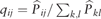}\right)}_{i,j}$ such that ⁠, and apply the t-SNE to learn a 2-D map that reflects the similarities q_ij as well as possible. We observe that the same type of cells group together well, while some of the different type of cells are mixed and difficult to be distinguished, which is also found when the other methods are used. Note that the embedded data points approximately lie around a sphere. This phenomenon is often observed when the input similarity matrix is doubly stochastic, which can resolve the crowding problem (Lu et al., 2016b).

Fig. 6.

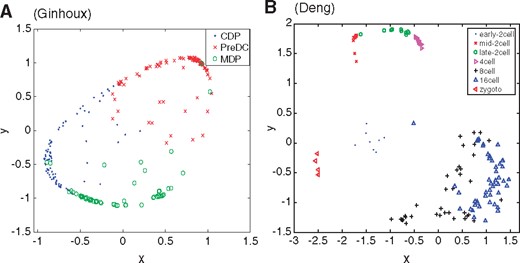
Visualization of the cells in 2-D spaces for Ginhoux (Schlitzer et al., 2015) (A) and Deng (Deng et al., 2014) (B) using the obtained $\widehat{P}$ of MPSSC. Different cell types are marked with different colors and shapes (Color version of this figure is available at Bioinformatics online.)

The second dataset (Deng et al., 2014), called Deng dataset in Table 1, consists of transcriptomes for individual cells isolated from mouse embryos at different preimplantation stages. The data consists of 135 cells and 12 548 genes, where cells belong to zygote, early 2-cell-stage, mid 2-cell-stage, late 2-cell-stage, 4-cell-stage, 8-cell-stage and 16-cell-stage. As seen in Figure 6B, MPSSC groups zygote, early 2-cell, mid 2-cell, late 2-cell and 4-cell stages quite well. However, the 8-cell and 16-cell stages could not be differentiated due to the technical variations of different library preparation protocols, which was also observed in Xu and Su (2015). This also can be explained by the fact that only a small number of genes have expression changes between the 8-cell and 16-cell (Hamatani et al., 2004; Wang et al., 2004). We note that for this data, MPSSC outperforms the other methods in all the three evaluation criteria, and none of the considered methods clearly distinguish the 8-cell and 16-cell populations.

5 Discussion

This article introduces a novel spectral clustering algorithm that imposes a specific structure on the target matrix, motivated by the observation that the target matrix should have this structure in the ideal case. We expect that imposing the ideal structure can help to achieve better clustering results, especially when the observed data include high levels of noise and many missing values. From various simulation and single-cell data analyses, we see the improved performance of our algorithm compared with the other clustering methods. The extended spectral clustering algorithm utilizing multiple similarity matrices can be favorable when the clusters have different densities and views. Theoretical analysis for the proposed clustering method in this setting will be our future work. For theoretical aspect, one might also try one-step spectral clustering method as in Remark 3, which has a simpler form. We solve the proposed non-convex problem iteratively with the embedded ADMM algorithm, and show the convergence of the algorithm. The convergence of the proposed algorithm is achieved only when c > 0, and using the appropriate c > 0 results in better clustering results than when c = 0. The topic of dealing with convergence of the algorithm without adding the term involving c will be of interest. Although we have demonstrated that finding valid values of λ and μ are usually not hard and altering these values in a certain range will not largely affect the results for many clustering problems, we expect that the optimal values of these parameters should depend on data and data-driven approaches for choosing these parameters will be of interest.

Funding

This work was supported in part by the National Institute of Health [GM59507, CA154295, CA196530].

Conflict of Interest: none declared.