Multiobjective multifactor dimensionality reduction to detect SNP–SNP interactions

Abstract

Motivation

Single-nucleotide polymorphism (SNP)–SNP interactions (SSIs) are popular markers for understanding disease susceptibility. Multifactor dimensionality reduction (MDR) can successfully detect considerable SSIs. Currently, MDR-based methods mainly adopt a single-objective function (a single measure based on contingency tables) to detect SSIs. However, generally, a single-measure function might not yield favorable results due to potential model preferences and disease complexities.

Approach

This study proposes a multiobjective MDR (MOMDR) method that is based on a contingency table of MDR as an objective function. MOMDR considers the incorporated measures, including correct classification and likelihood rates, to detect SSIs and adopts set theory to predict the most favorable SSIs with cross-validation consistency. MOMDR enables simultaneously using multiple measures to determine potential SSIs.

Results

Three simulation studies were conducted to compare the detection success rates of MOMDR and single-objective MDR (SOMDR), revealing that MOMDR had higher detection success rates than SOMDR. Furthermore, the Wellcome Trust Case Control Consortium dataset was analyzed by MOMDR to detect SSIs associated with coronary artery disease.

Availability and implementation: MOMDR is freely available at https://goo.gl/M8dpDg

Supplementary information

Supplementary data are available at Bioinformatics online.

1 Introduction

As revealed by the results of genome-wide association studies (GWAS), some diseases tend to be influenced by interactions between multilocus single-nucleotide polymorphisms (SNPs) (Moore et al., 2010). SNP–SNP interactions (SSIs) among genes have been found in some complex traits of the diseases (Steen, 2012). The analysts have considered SSIs as a solution to address concerns about missing heritability (Mackay, 2014). Moreover, developing efficient approaches for SSI analysis is imperative in genetic association studies (Mackay and Moore, 2014).

A model-free approach is one method which can be used to detect SSIs and does not require prior assumption of the genetic models and data. (Hahn et al., 2003; Li et al., 2014; Zhang et al., 2010). Multifactor dimensionality reduction (MDR) (Ritchie et al., 2001) is a well-known model-free approach in case–control studies. MDR entails adopting a dimensionality reduction technique to reduce the number of dimensions by converting a high-dimensional multilocus space into a one-dimensional space. It also entails using a two-way contingency table to assess SSIs and k-fold cross validation (CV) to avoid the overfitting of training data. MDR has been successfully applied in numerous disease and cancer studies, including oral cancer Yang et al., 2015c, hypertension (Yang et al., 2015a) and breast cancer (Fu et al., 2016).

Most of the extensions of MDR can be classified into three groups. The first group focuses on the modifications and combinations of biostatistics in terms of the uncertainty of binary high/low classification, such as odds ratio-based MDR (Chung et al., 2007), log-linear model-based MDR (Lee et al., 2007) and MDR-ER (Yang et al., 2013). The second group involves resolving particular data problems, such as quantitative MDR for quantitative traits (Gui et al., 2013) and Cox-MDR for survival data (Lee et al., 2012). Finally, the third group focuses on improving computational costs, such as unified model-based MDR (Yu et al., 2016), Fast MDR (Yang et al., 2015b), graphical processing unit (GPU)-based MDR (Greene et al., 2010) and differential evolution (DE)-based MDR (Yang et al., 2017). However, most MDR methods have been developed using a single measure based on a two-way contingency table [single-objective (SO) function] for SNPs and diseases. Considering the potential preference of measure-based approaches and the complexity of different disease models, (Bush et al., 2008) used classification error rate (CER) values to compare 10 measures based on a two-way contingency table; their results suggested that measures in MDR processes could substitute the likelihood rate (LR) for the CER. However, SOMDR may not operate satisfactorily in all disease models; i.e. certain solutions do not have the highest values for the CER and another measure. The CER conflicts with other measures in certain disease models; therefore, these measures cannot be easily incorporated in an MDR operation to detect SSIs. A multiobjective (MO) approach is a multiple-criteria decision analysis for explicitly evaluating multiple conflicting criteria in decisions (Greco et al., 2005). This approach enables n objectives to be evaluated simultaneously for obtaining agreeable solutions (Deb et al., 2014). An agreeable solution is referred to as a Pareto optimal solution, and a set of Pareto optimal solutions is called a Pareto set. The present study proposes an multiobjective MDR (MOMDR) method to incorporate two measures and obtain Pareto sets within k-fold CV. Therefore, more than one solution can be obtained in each CV. In CV consistency (CVC) operations, set theory is adopted to select optimal solutions (SSIs) from a number k of Pareto sets. We executed experiments on various simulation datasets and achieved satisfactory detection success rates. MOMDR was determined to have higher detection success rates and superior CVC, compared with SOMDR.

2 Approach

2.1 MDR process

MDR is a powerful data-mining tool for detecting non-linear interactions among multiple factors such as genetic (i.e. gene–gene or SNP–SNP) and environmental factors (Ritchie et al., 2001). A data reduction process is used to categorize the dimensionality of multilocus genotypes into high- and low-risk groups. This process enables transforming all multifactor combinations into a two-way contingency table. To avoid data overfitting, the k-fold CV approach was used to obtain k CV candidates. Subsequently, the CVC operation was performed to select an optimal solution from the k CV candidates. The MDR processes are detailed in the Supplementary Material.

2.2 MO function definition

For an MO maximization problem, the MO function can be formulated as max [f₁(x), …, f_n(x)], where the integer n ≥2 is the number of objectives and f: X →ℝⁿ, f(x) = [f₁(x), …, f_n(x)] is the set of objective functions. A decision vector is regarded as a solution to the problem of MO maximization, which is denoted as the vector x = (x₁, …, x_m), where m is the number of elements in x. A set X contains all feasible decision vectors (i.e. x ∈ X). If f_i(x₁) ≥ f_i(x₂) for all indices i ∈ {1, …, n}, then x₁ dominates another solution x₂. In the Pareto set X*, all vectors x* ∈ X* are not dominated by any other vector. For SSI detection, we considered an m-SNP combination (where m is the number of order SSI) as the decision vector and the measures as corresponding objective functions. For the consistency objective (maximize all objective functions), we select objectives’ correct classification rate (CCR; i.e. 1–CER) (Ritchie et al., 2001) and LR (Bush et al., 2008) to formulate the MO function as follows:

$$\text{Maximize}\{\begin{array}{c}{f}_1(x)=\text{CCR}(x)\\ f_2(x)=\text{LR}(x) \end{array}$$

(1)

where functions f₁ and f₂ are CCR and LR measures, respectively.

2.3 MOMDR process

In MOMDR, the Pareto set operation is included in the MDR process to simultaneously evaluate multiple objectives. Then, set theory is incorporated into the CVC operation for selecting optimal solutions. The Pareto set operation generates additional storage and applies Pareto-set filter operators to save all non-dominated solutions in each evaluation of the decision vector. For k-fold CV in the MDR process, the number k of Pareto sets (X*) is generated and initialized in an empty space. The elements in the Pareto sets can be improved throughout the evaluations of decision vectors. Therefore, each Pareto set among k-fold CV (X_j*, where j ∈ {1, …, k}) has more than one solution. Finally, the optimal solutions are selected by an intersection operation in the CVC operation. The training model in a fold of CV includes eight steps (Fig. 1):

Fig. 1.

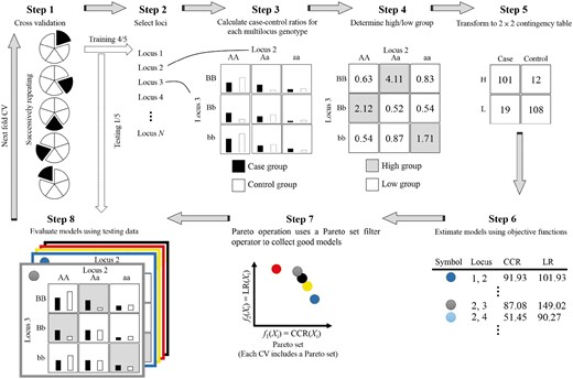
The procedure of MOMDR

• Step 1. The complete dataset is divided into a number of k subsets for CV. In the CV operation, a subset (j-subset, where j ∈ {1, _…, k}) is used as testing data, and the remaining subsets are used as training data. The CV operation uses the number of k training data to build models independently.

• Step 2. A set of all feasible decision vectors was generated and each decision vector (m-SNP combination) was evaluated by the following steps. According to the m-SNP combination, the numbers of m-combinations from a given dataset of n SNPs are generated to evaluate all SSIs. For example, the set of feasible decision vectors with two-SNP combinations from a dataset of 3 SNPs {S₁, S₂, S₃} is {{S₁, S₂}; {S₁, S₃}; {S₂, S₃}}.

• Step 3. A table of multifactor classes is generated, and the numbers of cases and controls in the classes are counted. SNPs typically have three genotypes; therefore, a decision vector can construct a table having 3^m multifactor classes. The samples in the training data are classified into multifactor classes according to genotype combinations, followed by counting of the numbers of cases (black bar, Fig. 1, Step 3) and controls (white bar).

• Step 4.1. The ratios between cases and controls in all multifactor classes are calculated using Equation (2).

  $$\widehat{{\theta }_a}=\frac{n_{+0}\times n_{a1}}{n_{+1}\times n_{a0}}$$

  (2)

where n_ab is the number of samples within the ath multifactor class in the b outcome [control (b = 0) and cases (b = 1)] and n_+b is the total number of samples in the b outcome [control (b = 0) and cases (b = 1)]. Equation (2) is an adjustment function to identify low- and high-risk groups to deal with unbalanced datasets (Yang et al., 2013).

• Step 4.2. The high- or low-risk groups in multifactor classes are determined. Each multifactor class is labeled as a low-risk group when the ratio $\widehat{{\theta }_a}$ (Equation 2) is <1 (Ritchie et al., 2001); otherwise, the class is labeled as a high-risk group. The labeled multifactor classes are referred to as the label table.

• Step 5. The number of 3^m labeled classes is transformed into a two-way contingency table according to groups (high- or low risk) and outcomes (cases and controls). Each cell in the two-way contingency table represents the number of samples (table in Step 3) belonging to the corresponding groups and outcomes (table in Step 4).

• Step 6. The objective functions within a feasible decision vector are evaluated. According to the MO function definition, two objective functions, which are based on the two-way contingency table, are considered to detect SSIs.

Objective 1: The CCR is the first objective function f₁(X_i) that calculates the proportion of correctly classified individuals within a feasible decision vector (Equation 3).

$$\begin{array}{c}{f}_1\left(X_i\right)=\text{CCR}\left(X_i\right)\\ =0.5\times \left(\frac{A}{A+C}+\frac{D}{B+D}\right)\end{array}$$

$$\text{s.t. }\{\begin{array}{c}A={\displaystyle \sum _{a\in \{\widehat{{\theta }_a},{\theta }_a\ge 1\}}{t}_{a1}}\\ B={\displaystyle \sum _{a\in \{\widehat{{\theta }_a},{\theta }_a\ge 1\}}{t}_{a0}}\\ C={\displaystyle \sum _{a\in \{\widehat{{\theta }_a},{\theta }_a<1\}}{t}_{a1}}\\ D={\displaystyle \sum _{a\in \{\widehat{{\theta }_a},{\theta }_a<1\}}{t}_{a0}}\end{array}$$

(3)

where t_ab is the set of individual matches to the ath multifactor class in the b outcome status, where b = 1 for the case group and b = 0 for the control group. A and B are the numbers of case and control samples classified into the high-risk group, respectively, and C and D are those classified into the low-risk group, respectively. To handle unbalanced datasets, the CCR function was used to determine the balanced accuracy using the A and D ratios for cases and controls, respectively (Yang et al., 2013), where the value is between 0 and 1; a value of 1 indicates the most optimal solution.

Objective 2: The LR is the second objective function f₂(X_i) (Equation 4) used in the MO function definition (Equation 1). The LR statistically compares the maximum likelihood of an unrestricted model, which consists of the observed frequencies in the data, with a restricted model, which comprises expected frequencies under the null hypothesis of no association (Bush et al., 2008).

$$\begin{array}{l}{f}_2\left(X_i\right)=\text{LR}\left(X_i\right)\\ =2\sum \text{Observed} \hspace{0.17em}\text{log}\hspace{0.17em} [\frac{\text{Observed}}{\text{Expected}}]\\ =2[A\times \text{log}\hspace{0.17em}\left(\frac{A}{A^{*}}\right)+B\times \text{log}\hspace{0.17em}\left(\frac{B}{B^{*}}\right)\\ +C\times \text{log}\hspace{0.17em}\left(\frac{C}{C^{*}}\right)+D\times \text{log}\hspace{0.17em}\left(\frac{D}{D^{*}}\right)]\end{array}$$

$$\mathrm{s}.\mathrm{t}. \{\begin{array}{c}{A}^{*}=\frac{\left(A+C\right)\left(A+B\right)}{A+B+C+D}\\ B^{*}=\frac{\left(B+D\right)\left(A+B\right)}{A+B+C+D}\\ C^{*}=\frac{\left(A+C\right)\left(C+D\right)}{A+B+C+D}\\ D^{*}=\frac{\left(B+D\right)\left(C+D\right)}{A+B+C+D}\end{array}$$

(4)

where A, B, C and D are the same as those in (Equation 3).

• Step 7. Pareto operation. The Pareto operation uses a Pareto-set filter operator to collect good solutions (X_j* = (x₁*, …, x_i*) in Pareto set_j, where j ∈ {1, …, k}) according to the MO values. All x* do not dominate one another in X_j*. The Pareto operation includes two steps: Step 1: Comparison between the decision vector X and all x* in X_j*; if X is not dominated by any x*, X is added to X_j*. Step 2: comparison between x_p and x_q (p ≠ q) in X_j*; if x_p is dominated by x_q, x_p is discarded from X_j* [i.e. f_i(x_q) ≥ f_i(x_p) for all indices i ∈ {1, …, n}, where n is the number of objective functions].

• Step 8. Each solution was evaluated on the basis of the testing data.

In aforementioned MOMDR process, Steps 1–8 are repeated until all feasible decision vectors are completely determined in each CV set. Following this iterative procedure, the number of k Pareto sets is obtained. In the CVC operation, the intersection operation was used to the select the optimal solutions. For each candidate, the number of occurrences in the Pareto sets is counted. The candidates with the highest CVC in all Pareto sets are considered as the optimal solutions. Finally, the medians of the objective values in the optimal solutions (evaluated in Step 8) are considered as the model measures using testing data.

3 Results

The performance of MOMDR was evaluated by comparing CCR- and LR-based MDR by using simulated datasets and a large genome-wide dataset from the Wellcome Trust Case Control Consortium (WTCCC; http://www.wtccc.org.uk/) using the Affymetrix GeneChip 500 K Mapping Array Set (Burton et al., 2007).

3.1 Experiments on simulated data

3.1.1 Case 1: disease loci with marginal effects

Disease loci with marginal effects were used to evaluate the performance of SOMDR and MOMDR in detecting disease-associated SSIs. We used six disease models with marginal effects (Namkung et al., 2009); disease Models 1–3 were obtained from (Namkung et al., 2009) and disease Models 4–6 were obtained from (Ritchie et al., 2003). The disease models were designed according to the interaction structure with different diseases, minor allele frequencies (MAFs), and prevalences. The details of the multilocus penetrances are presented in the Supplementary Table S1. The heritability (h²) values were between 0.031 and 0.008. In each disease model, 100 datasets were randomly generated using GAMETES, which can generate datasets containing a specific two-locus SSI with random architectures (Shang et al., 2013). Each dataset included an interacting SNP pair (M0P0 and M1P1) which was generated according to the disease model setting, and other SNPs were generated with an MAF selected uniformly in (0.05, 0.5). In case 1, our goal was to detect the interacting SNP pair (M0P0 and M1P1) in each dataset. The detection success rates were calculated by observing the frequency of goal detection within an epistatic model for each of the 100 datasets.

The detection success rates of SOMDR (CCR), SOMDR (LR), and MOMDR in the six models are presented in Figure 2 (white bar). The detection success rates of all methods could be improved by increasing the sample size. In general, SOMDR (LR) had higher detection success rates than SOMDR (CCR); however, Model 4 showed that SOMDR (CCR) had a higher detection success rate than SOMDR (LR). Our results are consistent with those of (Bush et al., 2008) at different simulation settings. The details of comparison between MOMDR and SOMDR (LR) in the six models with marginal effects are shown in Supplementary Table S2. MOMDR outperformed SOMDR (LR) in six models with marginal effects. The Wilcoxon signed-rank test was used to compare the performance of SOMDR and MOMDR in the six disease models (Table 1). A P value of < 0.05 (bold type) was considered to indicate significant superiority of MOMDR to the other methods. R⁻ represents the degree to which MOMDR is inferior to SOMDR, and the results demonstrated that MOMDR was superior to SOMDR. Moreover, MOMDR exhibited a significant improvement compared with SOMDR (R⁺), in which SOMDR (LR) had good detection success rates in the datasets with 800 samples. Regarding the detection success rates at CVC = 5, SOMDR (LR) outperformed SOMDR (CCR), particularly for disease Models 1, 2, 3, 5 and 6; this indicates that SOMDR (LR) exhibited improved stability in different datasets, but this stability may decline in certain disease models (e.g. disease Model 4). However, MOMDR had higher stability than SOMDR (LR) and SOMDR (CCR). Table 2 presents the Wilcoxon signed-rank test results for the detection success rate at CVC = 5. Although MOMDR and SOMDR (LR) had the same SSI detection ability in the dataset with 800 samples (Table 1), MOMDR outperformed SOMDR (LR) in terms of stability (CVC = 5). These results indicate that the MO approach can effectively detect SSIs because it can simultaneously consider multiple measures in disease loci with marginal effects.

Table 1.

Comparison of SOMDR and MOMDR for detection success rate using the Wilcoxon Signed-Rank test

MOMDR versus	R−	R+	R=	Mean rank	Sum of ranks	Z-test	P value
Case 1: 400 samples
CCR	0	6	0	3.5	21.0	−2.201	0.028
LR	0	6	0	3.5	21.0	−2.232	0.026
Case 1: 800 samples
CCR	0	5	1	3.0	15.0	−2.023	0.043
LR	0	1	5	1.0	1.0	−1.000	0.317
Case 2: 400 samples
CCR	0	23	17	12.0	276.0	−4.207	<0.001
LR	0	20	20	10.5	210.0	−3.933	<0.001
Case 2: 800 samples
CCR	0	10	30	5.5	55.0	−2.825	0.005
LR	0	15	25	8.0	120.0	−3.415	0.001
Case 3: 400 samples
CCR	0	4	4	2.5	10.0	−1.826	0.068
LR	0	5	3	3.0	15.0	−2.070	0.038
Case 3: 800 samples
CCR	0	5	3	3.0	15.0	−2.023	0.043
LR	0	5	3	3.0	15.0	−2.023	0.043

R⁻, negative ranks; R⁺, positive ranks; R⁼, ties; n, numbers, bold type indicates the significant improvement (P < 0.05).

Table 2.

Comparison of SOMDR and MOMDR for detection success rate in CVC = 5 using the Wilcoxon Signed-Rank test

MOMDR versus	R−	R+	R=	Mean rank	Sum of ranks	Z-test	P value
Case 1: 400 samples
CCR	0	5	1	3.0	15.0	−2.023	0.043
LR	0	3	3	2.0	6.0	−1.604	0.068
Case 1: 800 samples
CCR	0	6	0	3.5	21.0	−2.201	0.028
LR	0	6	0	3.5	21.0	−2.220	0.026
Case 2: 400 samples
CCR	0	31	9	16.0	496.0	−4.869	<0.001
LR	0	31	9	16.0	496.0	−4.886	<0.001
Case 2: 800 samples
CCR	0	14	26	7.5	105.0	−3.311	0.001
LR	0	20	20	10.5	210.0	−3.938	<0.001
Case 3: 400 samples
CCR	0	4	4	2.5	10.0	−1.826	0.068
LR	0	3	5	2.0	6.0	−1.633	0.102
Case 3: 800 samples
CCR	0	5	3	3.0	15.0	−2.060	0.039
LR	0	5	3	3.0	15.0	−2.023	0.043

R⁻, negative ranks; R⁺, positive ranks; R⁼, ties; n, numbers.

Fig. 2.

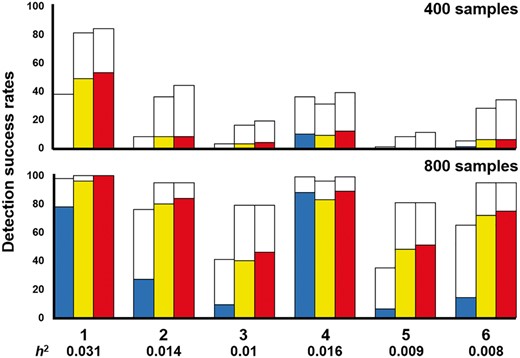
Comparison between SOMDR and MOMDR in the six disease models with marginal effects. For each disease model, the detection success rate was calculated as the proportion of 100 datasets, in which the specific SSI was detected. Each dataset included 1000 SNPs, and the sample sizes were 400 (200 cases and 200 controls, above figure) and 800 (400 cases and 400 controls, below figure). In each disease model, the bars from the left to the right indicate SOMDR (CCR), SOMDR (LR) and MOMDR. In each bar, the white region is the total detection success rate. The non-white regions represent the detection success rates of SOMDR (CCR), SOMDR (LR) and MOMDR at CVC = 5, respectively. The absence of bars indicates zero detection success rate

For 100 datasets including 1000 SNPs with 400 samples in disease loci with marginal effects, MOMDR took an average of 12.7 s to run a complete process, whereas SOMDR took an average of 12.4 s. For 800 samples, the average computational times of MOMDR and SOMDR were 28.1 and 27.3 s, respectively.

3.1.2 Case 2: disease loci without marginal effects

A total of 40 two-locus and pure disease models without marginal effects were obtained from (Wan et al., 2010). The simulation datasets were generated under various parameter settings (h² and MAF values) by using GAMETES. Each dataset contained a specific two-locus interacting SNP pair (M0P0 and M1P1) with random architectures (Urbanowicz et al., 2012). The details of the multilocus penetrances are presented in the Supplementary Tables S3–S6. The h² values that controlled the phenotypic variation of all disease models and ranged from 0.025 to 0.2, and MAFs of 0.2 and 0.4 were included. Each disease model was generated using 100 datasets consisting of 1000 SNPs, in which two SNPs (M0P0 and M1P1) were the specific SNPs, and other SNPs were generated with MAFs selected uniformly in (0.05, 0.5). The detection success rates were calculated by observing the frequency of goal detections through the datasets within a disease model (without marginal effects).

The detection success rates of SOMDR (CCR), SOMDR (LR) and MOMDR in the 40 disease models are presented in Figure 3. The detection success rates in disease models 11–40 could be improved by increasing the sample size. The results showed that SOMDR (LR) had higher detection success rates than SOMDR (CCR). The details of comparison between MOMDR and SOMDR (LR) in the 40 models without marginal effects are shown in Supplementary Table S7. MOMDR achieved superior results in 33 models among 40 models without marginal effects within 400 samples, and 22 models of MOMDR were superior to those of SOMDR (LR) within 800 samples; other models demonstrated equal detection success rates. The Wilcoxon signed-rank test was employed to compare the performance of SOMDR and MOMDR in the 40 disease models (Table 1). A p value of < 0.05 (bold type) was considered to indicate significant superiority of MOMDR to SOMDR (CCR) and SOMDR (LR).

Fig. 3.

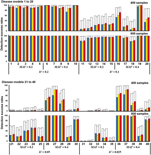
Comparison between SOMDR and MOMDR in the disease models without marginal effects. Under each setting, the detection success rate was calculated as the proportion of 100 datasets, in which the specific disease-associated SSIs were detected. Each dataset contains 1000 SNPs. In each disease model, the bars from the left to the right represent SOMDR (CCR), SOMDR (LR) and MOMDR. In each bar, the white region is the total detection success rate. The non-white and red regions represent the detection success rates of SOMDR (CCR), SOMDR (LR) and MOMDR at CVC = 5, respectively. The absence of bars indicates zero detection success rate

The results demonstrated that MOMDR was not inferior to SOMDR (R⁻), and that MOMDR exhibited significant improvement compared with SOMDR (R⁺). At CVC = 5, SOMDR (CCR) exhibited a high stability in disease Models 21–25 and 31–35, indicating that SOMDR (LR) may have decreased stability in certain disease models. However, MOMDR had higher stability than SOMDR (LR) and SOMDR (CCR). The Wilcoxon signed-rank test results for the detection success rate at CVC = 5 indicated that MOMDR showed significantly improved stability (Table 2). Therefore, the MO approach can effectively detect SSIs in disease loci without marginal effects.

For 100 datasets including 1000 SNPs with 400 samples in disease loci without marginal effects, MOMDR took an average of 12.7 s to run a complete process, whereas SOMDR took an average of 12.4 s. For 800 samples, the average computational times of MOMDR and SOMDR were 28.1 and 27.4 s, respectively.

3.1.3 Case 3: random simulation

We used GAMETES to generate 100 000 random, strict, and pure disease models for each of the different combinations of genetic constraints that were obtained using different two-locus interacting SNP pairs (M0P0 and M1P1); h² values of 0.001, 0.025, 0.05 and 0.1; and MAFs of 0.2 and 0.4, with a varying population prevalence. For each setting, 100 000 disease models were ranked on the basis of the ease of detection measure (EDM), and the disease models with the lowest EDM values were selected as the random disease models for data simulation (Urbanowicz et al., 2012). For each selected disease model, we simulated 100 replicate datasets under the sample sizes of 400 and 800 with balanced cases and controls and a total of 1000 SNPs. Each dataset contained one pair of highly interactive SNPs (M0P0 and M1P1), and other SNPs were generated with MAFs selected uniformly in (0.05, 0.5). The detection success rates were calculated by observing the frequency of goal detection through the datasets within the random disease models.

The detection success rates of SOMDR (CCR), SOMDR (LR) and MOMDR in the eight random disease models are illustrated in Figure 4. For all disease models, the detection success rates in Methods 1, 2 and 5 revealed that SOMDR (LR) had higher detection success rates than SOMDR (CCR); however, SOMDR (LR) was inferior in disease Models 6 and 7. The details of comparison between MOMDR and SOMDR (LR) in the eight random models are shown in Supplementary Table S8. MOMDR outperformed SOMDR (LR) when the MAF = 0.4 and h² < 0.05 (Models 1, 2, 3, 4, 6 and 8), in which the increased MAF and decreased h² values experienced more difficulty detecting the goal (the particular SSI). The Wilcoxon signed-rank test indicated that MOMDR was significantly superior to SOMDR (CCR) and SOMDR (LR). In addition, R⁻ was not observed in all disease models, and MOMDR had higher detection success rates than SOMDR (R⁺). At CVC = 5, the results indicated that SOMDR (LR) had a higher stability than SOMDR (CCR) in the disease models; nevertheless, SOMDR (LR) had lower detection success rates in disease Models 6 and 7. MOMDR had higher stability than SOMDR (LR) and SOMDR (CCR). The Wilcoxon signed-rank test results for the detection success rate at CVC = 5 indicated that MOMDR exhibited significantly improved stability compared with SOMDR (CCR) and SOMDR (LR) (Table 2). Therefore, MOMDR can be effective in SSI detection in the random disease models.

Fig. 4.

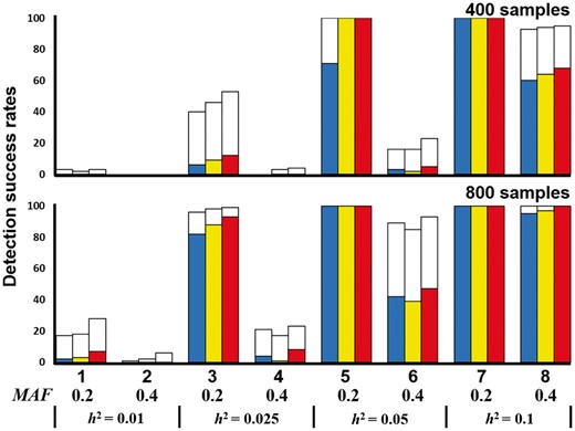
Comparison between SOMDR and MOMDR in the random disease models. Under each setting, the detection success rate was calculated as the proportion of 100 datasets, in which the specific disease-associated SSIs were detected. Each dataset contains 1000 SNPs. In each disease model, the bars from the left to the right represent SOMDR (CCR), SOMDR (LR) and MOMDR. In each bar, the white region is the total detection success rate. The non-white regions represent the detection success rates of SOMDR (CCR), SOMDR (LR) and MOMDR at CVC = 5, respectively. The absence of bars indicates zero detection success rate

For 100 datasets including 1000 SNPs with 400 samples in a random simulation, MOMDR took an average of 12.8 s to run a complete process, whereas SOMDR took an average of 12.5 s. For 800 samples, the average computational times of MOMDR and SOMDR were 28.1 and 27.3 s, respectively.

3.2 Experiments on the WTCCC dataset

A real dataset was obtained from the WTCCC to evaluate MOMDR performance. The dataset was collected through a collaborative effort between 50 British research groups established in 2005 (Burton et al., 2007) and contains a total of 500 569 SNPs, including 1988 cases with coronary artery disease (CAD) and 1500 controls obtained from people living in Great Britain who self-identified as white Europeans. These people were genotyped using the Affymetrix GeneChip 500 K Mapping Array Set.

Supplementary Table S9 shows the SSIs detected by MOMDR. The SNP locations were determined from dbSNP at the National Center for Biotechnology Information (https://www.ncbi.nlm.nih.gov/snp/). The designation UNKNOWN’ in the table refers to an SNP that is not located on a gene. Each chromosome includes more than one detected SSI because MOMDR yields more than one solution. The P-values were calculated through a chi-squared (χ²) test using the raw datasets to determine the significance level for an epistatic interaction between the two SNPs. All SSIs detected by MOMDR in the 24 chromosomes yielded P < 0.0001, indicating a highly significant interaction between the two SNPs. The CVC shows the degree to which the same best model is discovered across five divisions of the data, and CVC = 5 indicates the highest degree (Motsinger and Ritchie, 2006). When the CCR was higher than 0.5, the frequency of chance was significantly reduced, indicating that our results identified significant SSIs (Coffey et al., 2004). High LR values indicate that uncertainties were reduced in the disease model (Bush et al., 2008). The CCR values were in the range of 0.675–0.988, with the mean CCR value being 0.787 [SD = 0.086]. The LR values were in the range of 39.2–724.4, with the mean LR value being 211.2 (SD = 163.7). Notably, the SSIs rs1454640 and rs3989940 (Chromosome 12) achieved the highest CCR (0.988) and LR (724.4) values (CVC = 5, P < 0.0001, marked by a double asterisk in Supplementary Table S9). The six detected SSIs thus demonstrate the beneficial measures of LR > 400 and CCR > 0.9 (CVC = 5, P < 0.0001, marked by asterisks in Supplementary Table S9). These seven SSIs showed high values of CCR (>0.9), LR (>400) and CVC (=5) and strong significance (P < 0.0001), indicating these SNP pairs could potentially be the epistatic interactions in CAD. Further studies on implicated genes polymorphisms and their functional relevance could provide crucial information for the etiology and treatment of CAD. The running times of chromosomes in the WTCCC dataset are shown in Supplementary Table S9. Regarding the average running times for all large datasets, both SOMDR and MOMDR required ∼6.16 h, indicating that MOMDR does not increase the running time.

4 Discussion

According to our review of the relevant literature, this study is the first to implement an MO approach-based MDR for SSI detection. In the MDR process, a combination of high-dimensional factors can be reduced by assigning multilocus genotypes to high- or low-risk groups, enabling the determination of SSI quality through two-way contingency table analysis (Ritchie et al., 2001). The CCR is the most commonly applied measure in MDR-based methods (Gola et al., 2016). Bush et al. (2008) compared 10 general measures in the text classification field to evaluate the degree of improvement in the SSI detection ability of MDR; the LR was suggested to improve MDR detection in simulations. Our results also demonstrated that SOMDR (LR) revealed a detection ability superior to that of SOMDR (CCR) in all of the tests. The success of MOMDR is primarily attributed to the conflicts between CCR and LR measures in certain disease models, which increase the detection success rates. In three experiments on simulated data, SOMDR (LR) did not outperform SOMDR (CCR) in all disease models, indicating that an optimal known solution could either have the highest LR or CCR value. These disease models could be detected using either the LR or CCR measure. Moreover, the optimal solution may have the highest value in one measure and not have appreciable values in the other measure in all feasible decision vectors. This situation indicates that the CCR is usually one of the main criteria, but it may conflict with the other measure (Greco et al., 2005). Therefore, the CCR and other measures (e.g. the LR) do not equally contribute to increased SSI detection ability. MOMDR can simultaneously evaluate multiple measures for detecting SSIs. It exhibited the most successful SSI identification rates when the LR and CCR were used simultaneously to determine significant SSIs in this study.

The detection of disease-associated SNPs was considerably complex in the current case–control study. A single measure may not be able to detect some vital SSIs, thus, multiple measures should be used to successfully detect significant associations, and even enhance the credibility of the result. MOMDR was enabled to simultaneously employ multiple measures to determine potential SSIs. The results demonstrated that MOMDR performed strongly in both simulated and real datasets. Moreover, MOMDR retained the following advantages of MDR methods. First, MOMDR can handle unbalanced datasets (i.e. situations in which the numbers of cases and controls are different). MOMDR uses adjustment functions (Eqs. 2 and 3) to identify low- and high-risk groups and to evaluate the SSIs for selecting the optimal solutions for unbalanced datasets. Therefore, MOMDR can accurately classify multiple classes into high- and low-risk groups and subsequently increase the values of A and D in Equation (3). Second, MOMDR can effectively minimize false-positive results to detect SSIs. MOMDR uses the CV function to select optimal solutions solely based on its ability to make predictions using independent data. This is an important model validation technique to avoid data overfitting and reduce false positives in statistical analysis. Third, MOMDR can describe the locus genotype combinations associated with high- and low-risk disease groups. Through the reduction of the dimensionality of the multilocus data, the simultaneous detection of multiple genetic loci associated with diseases can be clearly identified to determine whether they are more common in affected or unaffected individuals. Fourth, MOMDR is a model-free method, which does not require a specific mode of inheritance (Ritchie et al., 2001). In human physiology, epistasis is chaotic and irreducible, with gradual changes with an unknown mode of inheritance. However, there are simple mono- or oligo-genetic traits that might relate to the epistasis. Therefore, the model-free method is very crucial for detecting SSIs to understand epistasis. In addition, MOMDR can be used directly for case–control and family-based control studies. Finally, MOMDR is non-parametric, rendering it suitable for use with small samples; thus, it is widely applied in the tests of differences between independent samples (e.g. case–control studies). Non-parametric methods are not required to assume the distribution of data before statistical analysis, and they can thus avoid problems associated with the use of parametric statistics to detect high-order epistatic interactions (Ritchie et al., 2001).

Currently, many MDR studies focus on addressing the problems facing multilocus modeling (Gola et al., 2016) to overcome statistical challenges, including population stratification, cryptic relatedness, differential linkage disequilibrium and haplotype effects. In this study, we do not address the statistical limitations of MDR, because MOMDR is based on the original multilocus modeling of MDR. Our MOMDR can be incorporated with adjusted MDR methods because most MDR versions must use the measurement required to evaluate SSIs in the transformed 2 × 2 contingency table. Niu et al. (2011) used the principal components of genotypes at a set of unlinked markers to represent the genetic background. Then, the genetic background was used to control the population stratification. Thus, an association test based on the principal components of genotypes was employed (instead of using the ratio of cases to controls as MDR does) to classify the multilocus genotype as high- or low-risk in each multilocus cell. Lee et al. (2007) mixed the log-linear models to reclassify the cells with the best combination of factors. The expected number of cases and controls per cell are calculated using maximum likelihood estimates of the selected log-linear models. Thus, the expected numbers can be used to classify the multilocus genotype as high- or low-risk. In future applications of MOMDR in studies of genetic interactions, a more conservative outcome can be achieved in potentially high-risk epistasis to avoid excessive Type I errors (false positive). Furthermore, in applications, MOMDR might be limited to the datasets that are genetically homogeneous. Further exploration of the possible impacts of batch effects on analyses is required.

Regarding implemental efficiency, MOMDR is similar to SOMDR. For 100 datasets including 1000 SNPs with 800 samples, MOMDR was determined to spend on average 28.1 s to run a complete process on an Intel Core i7 2.8 GHz CPU with 4 GB memory, whereas SOMDR spent on average 27.3 s. To determine the optimal n-locus models among the number of k subsets in the number of m SNPs, MOMDR would require a total computational time of k × (m choose n) × the total number of samples × 3ⁿ times. Moreover, the computational time can be improved by adopting powerful computation approaches such as parallel operations (Bush et al., 2006), GPU-based MDR (Greene et al., 2010), the greedy search strategy (Yang et al., 2015b) and DE-based MDR (Yang et al., 2017).

In MDR-based methods, certain SSIs can be detected using particular measures such as the CCR and LR based on a two-way contingency table. The MO approach enables MOMDR to generate several SSI sets from multiple measures based on the two-way contingency table. Therefore, each fold of CV includes at least one candidate in k-fold CV, and our improved CVC operation can systematically predict the optimal SSIs among multiple candidates. The MOMDR performance assessment revealed that the applied MO approach was successful in enhancing MDR method’s detection success rates for SSIs. The WTCCC analysis revealed that MOMDR can detect several significant SSIs. In future studies, additional measures based on a two-way contingency table can be combined and flexibly embedded into MOMDR to enhance detection ability.

Acknowledgements

We thank editor Oliver Stegle and reviewers for their help and comments during preparation of the article.

Funding

This work was partly supported by the Ministry of Science and Technology, R.O.C. [grant no. 105-2221-E-151 -053 -MY2 and 106-2811-E-151-002-].

Conflict of Interest: none declared.