Dissecting newly transcribed and old RNA using GRAND-SLAM

Abstract

Summary: Global quantification of total RNA is used to investigate steady state levels of gene expression. However, being able to differentiate pre-existing RNA (that has been synthesized prior to a defined point in time) and newly transcribed RNA can provide invaluable information e.g. to estimate RNA half-lives or identify fast and complex regulatory processes. Recently, new techniques based on metabolic labeling and RNA-seq have emerged that allow to quantify new and old RNA: Nucleoside analogs are incorporated into newly transcribed RNA and are made detectable as point mutations in mapped reads. However, relatively infrequent incorporation events and significant sequencing error rates make the differentiation between old and new RNA a highly challenging task. We developed a statistical approach termed GRAND-SLAM that, for the first time, allows to estimate the proportion of old and new RNA in such an experiment. Uncertainty in the estimates is quantified in a Bayesian framework. Simulation experiments show our approach to be unbiased and highly accurate. Furthermore, we analyze how uncertainty in the proportion translates into uncertainty in estimating RNA half-lives and give guidelines for planning experiments. Finally, we demonstrate that our estimates of RNA half-lives compare favorably to other experimental approaches and that biological processes affecting RNA half-lives can be investigated with greater power than offered by any other method. GRAND-SLAM is freely available for non-commercial use at http://software.erhard-lab.de; R scripts to generate all figures are available at zenodo (doi: 10.5281/zenodo.1162340).

1 Introduction

Gene expression is a highly dynamic process and determined by the interplay of RNA transcription, processing and decay (Schwanhausser et al., 2011). High-throughput techniques such as microarray and next generation sequencing (NGS) have become standard tools to quantify gene expression on the level of total RNA. However, knowing the amount of total RNA for each gene at the time of cell lysis does not provide information to distinguish between the processes that constitute gene expression. For instance, when gene expression changes between some treatment and control condition are investigated, differences between total RNA levels can arise due to the treatment affecting transcription, processing or decay. Moreover, if changes after a short period of time (e.g. 1 h after infection by a virus) are of interest, considering total RNA levels can be heavily misleading (Marcinowski et al., 2012).

To resolve these issues, powerful biochemical approaches have been developed in recent years. Most successfully, newly transcribed RNA can be metabolically labeled using nucleoside analogs such as 4-thiouridine (4sU) in living cells. After RNA extraction, labeled RNA can be biochemically separated from pre-existing, unlabeled RNA by thiol-specific biotinylation. Both fractions, in addition to total RNA, can be quantified using microarrays or RNA sequencing. This has allowed to precisely measure RNA half-lives (Dölken et al., 2008), monitor RNA splicing (Windhager et al., 2012) or investigate extremely short-lived RNAs (Schwalb et al., 2016) or complex regulatory processes (Rabani et al., 2014). However, the biochemical separation step is laborious and error-prone, and requires large amounts of RNA. Moreover, imperfect biochemical separation may introduce severe bias and bioinformatic analysis such as data normalization is highly challenging (Uvarovskii and Dieterich, 2017).

Recently, three studies introduced an alternative approach to differentiate between new and old RNA: SLAM-seq (Herzog et al., 2017), Timelapse-seq (Schofield et al., 2018) and TUC-seq (Riml et al., 2017) directly visualize labeled RNA by sequencing: After labeling by 4sU and extraction of RNA, chemical agents are used to convert 4sU to cytosine analogs. The sample is sequenced without prior separation, and old and new RNA can be differentiated on the basis of specific T to C mismatches of reads mapped to the reference transcriptome. Importantly, the accuracy of this bioinformatic separation strongly depends on the error rates of sequencing and the 4sU incorporation rates. Even with very long periods of labeling (24h) and high concentrations of 4sU (100 μM), no more than one in 40 uridines is substituted by 4sU (Dölken et al., 2008; Herzog et al., 2017). Thus, only a small fraction of sequencing reads will contain more than one conversion. Moreover, the error rates of modern NGS dropped below 0.1%, but still give rise to many reads with T to C mismatches. Thus, it is not possible to decide with certainty for each individual read whether it originated from a new or an old RNA molecule.

Therefore, the computational approach termed SLAM-DUNK (Herzog et al., 2017) utilizes all observed T to C mismatches of reads mapped to a gene, and subtracts the observed mismatches from a control experiment without 4sU labeling. These corrected conversion rates were used to compute RNA half-lives in pulse-chase experiments: Efficient 4sU incorporation is achieved by long periods of labeling, followed by wash-out of free 4sU and monitoring the drop of corrected conversion rates over several time points. In addition, labeling for 3 h and 12 h was sufficient to reveal changes of RNA half-life induced by microRNAs and N⁶ adenosine methylation of the mRNAs in differential experiments, e.g. by knocking out an essential factor for microRNA biogenesis and comparing corrected conversion rates between knock-out and wild-type cells.

Here, we expand on this methodology and present the computational approach Globally refined analysis of newly transcribed RNA and decay rates using SLAM-seq (GRAND-SLAM) that allows to infer the proportion and the corresponding posterior distribution of new and old RNA for each gene in a single SLAM-seq experiment. Compared to the corrected conversion approach, it provides five major advantages: First, no control experiment is needed. Second, a single labeling experiment (as compared to a pulse-chase timecourse) is in principle sufficient to estimate RNA half-lives. Naturally, more experiments increase the accuracy of the estimate. Third, by directly utilizing the posterior distributions, estimated half-lives are more accurate. Fourth, the variance of the posterior distribution, or, alternatively, the size of credible intervals, provide an internal quality control for each gene and experiment. Finally, and most importantly, knowing the proportion of new RNA for each gene allows to investigate fast regulatory processes such as induced by virus infection, which is not possible when only knowing corrected conversion rates.

2 Approach

Our approach is based on a binomial mixture model (Fig. 1):

$$P(y;p_e,p_c,n,{\pi }_g)=(1-{\pi }_g)B(y;n,p_e)+{\pi }_{g}B(y;n,p_c)$$

(1)

$$B(k;n,p)=\left(\begin{array}{c}n\\ k\end{array}\right)·p^k{(1-p)}^{n-k}$$

(2)

Fig. 1.

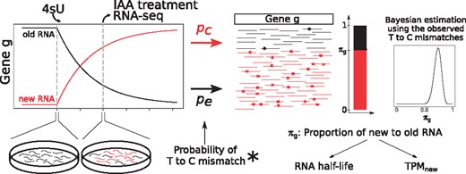
GRAND-SLAM overview. After a period of labeling with 4-thiouridine (4sU), RNA is extracted from cells, treated with IAA and sequenced. Shown is a theoretical timecourse of the abundances of new and old RNA for a gene g. IAA converts incorporated 4sU into cytosine analogs with an overall rate p_c (including the incorporation rate, conversion rate and error rate), and uridines are sequenced as cytosine with an error rate p_e. Based on the observed mismatches from T to C, the proportion of new to old RNA of gene g, π_g, can be estimated using Bayesian inference. Estimates of π_g can be transformed into estimates of the gene’s RNA half-life or relative abundance measures

The sufficient statistics for this model are the number of observed T to C mismatches (y) for each read mapped to a genomic region containing n thymines within a gene g. If π_g is the fraction of newly transcribed RNA among all RNAs of gene g, p_e is the average T to C mismatch rate in unlabeled RNA and p_c is the average mismatch rate in labeled RNA, then observed mismatches for a read are either due to a binomial distribution with success probabilty p_e (with probability $1-{\pi }_g$⁠) or a binomial distribution with success probability p_c (with probability π_g).

Thus, our goal is to estimate all π_g using Bayesian inference for observed data $\mathbf{y}=y_1,\dots ,y_m$ and $\mathbf{n}=n_1,\dots ,n_m$ (i.e. for each read, how many of the potential T to C mismatches have been observed):

$$f({\pi }_g;\mathbf{y},\mathbf{n},p_e,p_c)=\frac{\prod _{i}P(y_i;p_e,p_c,n,{\pi }_g)·b({\pi }_g;\alpha ,\beta )}{P\left(\mathbf{y}\right)}$$

(3)

For the sake of simplicity, we use a beta prior with density function b and hyperparameters α and β. As we have no prior knowledge on the proportion for each gene, we here use the uninformative uniform prior with $\alpha =\beta =1$⁠. In the denominator, the integral $P\left(\mathbf{y}\right)={\int }_0^{\mathrm{1}}\prod _{i}P(y_i;p_e,p_c,n,{\pi }_g^{\prime })·b({\pi }_g^{\prime };\alpha ,\beta )d{\pi }_g^{\prime }$ is computed numerically.

Here, we assume p_e and p_c to be constant throughout a sample. Thus, before solving Equation (3) for each gene, we estimate p_e and p_c based on the data from all genes.

3 Materials and methods

3.1 Sufficient statistics

The sufficient statistics for parameter estimation are collected in a matrix $A^{\left(g\right)}$⁠. Each entry $a_{k,n}^{\left(g\right)}$ is the number of reads mapped to a genomic region within gene g containing n thymines with k observed T to C mismatches. We only consider reads consistently mapped to a known transcript (i.e. matching all intron boundaries). Alternatively, for the SLAM-seq experiments (Herzog et al., 2017) where 3’ ends of transcripts are sequenced, we only consider reads mapped to the 3’ regions defined by SLAM-DUNK (Herzog et al., 2017). In addition we identify and exclude potential SNPs defined as thymines where more than half of the reads covering it show a mismatch.

3.2 Estimating p_e

In principle, p_e can be directly estimated from either spike-in RNAs in the same sample, or using an additional sample without 4sU labeling (no4sU sample) by counting T to C mismatches. However, utilizing an additional experiment may lead to a bad estimate for the 4sU sample of interest, as a broad range of p_e values is observed already in available no4sU samples (Fig. 4C). However, we noticed that the other eleven error rates (one of the nucleotides to any of the other three) are highly correlated to the T to C error rate in the no4sU samples. Thus, we trained a linear regression model to predict the T to C error rate from the other error rates. Manual feature selection revealed that the T to A and T to G error rates alone provided sufficent prediction performance in a leave-one-out cross validation for the datasets used in this study. Consequently, we used the linear regression model based on these two features here (Fig. 4D), but our implementation can handle any linear regression model or, alternatively, estimates from spike-in RNA.

3.3 Estimating p_c

To estimate p_c, we first compute $A=\left(a_{k,n}\right)=\sum _g{A}^{\left(g\right)}$⁠. Since y = 0 is the mode of both component distributions of the binomial mixture model, standard approaches to estimate p_e and p_c based on the expectation maximization (EM) algorithm failed. However, as we can assume that p_e < p_c, there is a certain k where only a minor fraction of reads with at least k T to C mismatches originates from the p_e component. This k can be computed for each n such that less than 1% of the observed reads with $\ge k$ mismatches is expected to originate from unlabeled RNA. Thus, for each n and k we compute

$$e_{k,n}=B(k;n,p_e)·\sum _{k\prime }{a}_{k\prime ,n}$$

(4)

and exclude (k, n) if $e_{k,n}>0.01a_{k,n}$⁠. More than 99% of the remaining $a_{k,n}$ originate from the p_c component, allowing to estimate p_c using an EM algorithm that treats the excluded $X=\left\{(k_1,n_1),\dots \right\}$ as missing data. If enough reads (we used 10 000 reads as threshold) remain, which was the case in all datasets but the 45 min labeling experiments from Herzog et al. (2017), p_c can be estimated with sufficient precision. Otherwise, our implementation stops with an error. Importantly, this will only happen when extremely few labeled RNA was in the sample.

The E step consists of replacing excluded read counts by their expected values given the current estimate $p_c^{\left(t\right)}$⁠:

$$a_{k,n}^{(t+1)}=\frac{\sum _{(k\prime ,n)\notin X}B(k;n,p_c^{\left(t\right)})·a_{k\prime ,n}}{\sum _{(k\prime ,n)\notin X}B(k\prime ;n,p_c^{\left(t\right)})}$$

(5)

The M step computes a better estimate for p_c as

$$p_c^{(t+1)}=\frac{\sum _{k,n}k{a}_{k,n}^{(t+1)}}{\sum _{k,n}n{a}_{k,n}^{(t+1)}}$$

(6)

We noticed that running the EM algorithm led to extremely slow convergence rates. Thus, we use the following bisection scheme instead: For the search interval $[l,r]$ (starting with l = 0 and r = 1), we set $p^{\left(t\right)}=\frac{l+r}{2}$ and compute $p^{(t+1)}$ by a single EM iteration. If $p^{(t+1)}<p^{\left(t\right)}$⁠, we continue with the search interval $[l,p^{\left(t\right)}]$⁠, otherwise with $[p^{\left(t\right)},r]$⁠. We stop if $r-l<{10}^{-8}$⁠.

3.4 Estimating the posterior

In principle, we compute the integral by dividing $[0,1]$ into k equisized intervals and employ Newton–Cotes quadrature using the trapezoidal rule. This also gives straight-forward access to any credible interval. To allow for relatively small k even for potentially extremely narrow posterior distributions f, we first identify the mode m of f by numerically maximizing

$$g({\pi }_g;\mathbf{y},\mathbf{n},p_e,p_c)=\sum _i\hspace{0.17em}\text{log}\hspace{0.17em}\left(P(y_i;p_e,p_c,n,{\pi }_g)\right)+\hspace{0.17em}\text{log}\hspace{0.17em}b({\pi }_g;\alpha ,\beta )$$

(7)

Then, we identify the values l < m, where $f\left(l\right)={10}^{-3}f\left(m\right)$ and h > m where $f\left(h\right)={10}^{-3}f\left(m\right)$ by bisection. The interval $[l,h]$ contains most of the probability mass, so we use this interval for the numerical integration.

Finally, we noticed that the posterior distribution for any gene g closely resembles a beta distribution with density b_g. Importantly, having a closed-form representation for the posterior is important for subsequent steps. Therefore we fit parameters α_g and β_g by numerically minimizing the sum of squares computed between f and b_g for all Newton–Cotes points.

3.5 Estimating RNA half-life

For the abundance a of an RNA with transcription rate σ and decay rate δ, the change over time is modeled by the following differential equation:

$$\frac{da}{dt}=\sigma -\delta a\left(t\right)$$

(8)

With an initial abundance a₀, this has the following closed-form solution:

$$a\left(t\right)=\left(a_0-\frac{\sigma }{\delta }\right){\mathrm{e}}^{-t\delta }+\frac{\sigma }{\delta }$$

(9)

Setting the intial abundance to zero for newly synthesized RNA and to the steady state for pre-existing RNA, we obtain the following functions for the abundance of new RNA a_new and old RNA a_pre:

$$a_{\text{new}}\left(t\right)=-\frac{\sigma }{\delta }{\mathrm{e}}^{-t\delta }+\frac{\sigma }{\delta }$$

(10)

$$a_{\text{pre}}\left(t\right)=\frac{\sigma }{\delta }{\mathrm{e}}^{-t\delta }$$

(11)

Thus, at any time t, the proportion of new to old RNA is

$$\pi \left(t\right)=\frac{a_{\text{new}}\left(t\right)}{a_{\text{new}}\left(t\right)+a_{\text{pre}}\left(t\right)}=1-{\mathrm{e}}^{-t\delta }$$

(12)

This can be used to transform the decay rate into a proportion π at time t and vice-versa:

$${\delta }_t(\pi )=-\frac{1}{t}\text{log}\hspace{0.17em}(1-\pi )$$

(13)

$${\pi }_t(\delta )=1-{\mathrm{e}}^{-t\delta }$$

(14)

Hence, for gene g if at any time t, the proportion of new and old RNA is an approximately beta distributed random variable ${\mathcal{P}}^{\left(t\right)}\sim \text{Beta}(\alpha ,\beta )$ with density function $b_g(\pi ;\alpha ,\beta )$⁠, the density function $d(\delta ;\alpha ,\beta )$ of the distribution of the transformed random variable ${\mathcal{D}}^{\left(t\right)}={\delta }_t\left({\mathcal{P}}^{\left(t\right)}\right)$ can be found by substitution:

$$d(\delta ;\alpha ,\beta )=b_g\left({\pi }_t(\delta );\alpha ,\beta \right)\frac{d{\pi }_t}{d\delta }$$

(15)

$$=\frac{t}{B(\alpha ,\beta )}{\left(1-{\mathrm{e}}^{-t\delta }\right)}^{\alpha -1}·{\mathrm{e}}^{-t\beta \delta }$$

(16)

Thus, if several approximate posterior beta densities defined by $({\alpha }_1,{\beta }_1),\dots ,({\alpha }_n,{\beta }_n)$ for proportion parameters measured at times $t_1,\dots ,t_n$ are given, the maximum a posteriori (MAP) estimator for the decay rate δ can be found by numerically maximizing:

$$l(\delta )=\sum _i({\alpha }_i-1)\hspace{0.17em}\text{log}\hspace{0.17em}(1-{\mathrm{e}}^{-t_i\delta })-t_i{\beta }_i\delta$$

(17)

Finally, the estimated decay rate δ can be transformed into an estimate of the RNA half-life λ by

$$\lambda =\frac{\hspace{0.17em}\text{log}\hspace{0.17em}\left(2\right)}{\delta }$$

(18)

3.6 Simulation

We utilized the available SLAM-seq data from Herzog et al. (2017) to determine realistic parameters for simulation. Specifically, we downloaded the processed table of a random sample (GSM2666852) from GEO and converted the CPM (read counts per million) into a read count distribution for genes by multiplying all CPM values by 20 million. Next, we downloaded the table containing half-lives estimated from their pulse-chase experiment and applied Equations (18) and (14) to derive a realistic distribution of new to old proportions for a putative experiment with 3 h 4sU labeling.

Data for Figure 2 were simulated by the following procedure: We simulated as many genes as in the read count distribution. For each gene, we randomly sampled a read count from this distribution and a π_g from the proportion distribution (except for Fig. 2B, where we set ${\pi }_g=0.5$ for all genes). For each read, we first sampled the total number of thymines n from a binomial distribution with parameters L (read length, here L = 50 as in the available experiments) and u [thymine content, here we set u = 0.3 as computed from the 3’ end investigated by Herzog et al. (2017)]. Then, we determined whether this read originated from a new RNA (with probability π_g) or old RNA (with probability $1-{\pi }_g$⁠). Finally, the number of T to C mismatches k was drawn from a binomial distribution with parameters n and either p_e or p_c (here we set $p_e=1\times {10}^{-4}$ and $p_c=0.023$⁠, compare Fig. 4).

Fig. 2.

Validation by simulation. (A) Estimation accuracy for the conversion rate p_c is shown as the deviation of the estimated value from the true value in percentage of the true value. The error rate p_e must be known to estimate p_c. Either the true error rate (Known p_e) is supplied to the algorithm, or the true error rate plus a normally distributed error [according to parameters inferred from the no4sU experiments from Herzog et al. (2017), Fig. 4C; Estimated p_e] (B) 90% credible intervals and the posterior means for the proportion parameter π_g are shown for 70 randomly sampled simulated genes. Here, the true p_c and p_e have been supplied to estimate. (C) Cumulative distributions of the absolute deviation from the true proportion are shown for all 18.917 simulated genes split by their read count n. Distributions for 100 simulations are overlayed. (D) The percentage of genes within equal-tailed credible intervals (CI; x-axis) is shown for all 18.917 simulated genes split by their read count n. As in (C) 100 simulations are overlayed

Reads for Figure 3 were generated in a similar manner, but here we directly selected a random read location from the gene 3’ regions defined by Herzog et al. (2017) and generated mismatches accordingly (all 12 possible mismatches with rate p_e or p_e when appropriate). Here, a fixed ${\pi }_g=0.2$ was used. Read locations were either directly written to a read mapping file, or sequences were generated and written to fastq files.

Fig. 3.

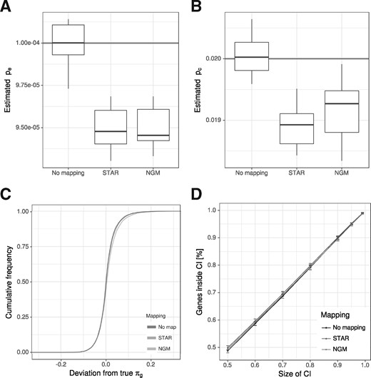
Influence of read mapping. (A and B) We simulated 10 datasets of reads and either used the true locations of the reads (No mapping) as input for GRAND-SLAM, or a fastq file for STAR or NGM. Here, the distributions of the estimated error rates (A) and conversion rates (B) are shown. The true values are indicated. Read mapping with both STAR and NGM led to slighly, but significantly biased estimates. (C) The cumulative distribution of the absolute deviation from the true proportion is shown for reliably quantified genes (at least 100 reads). In spite of underestimated rates, read mapping effects on estimating the proportion are neglibible. (D) The percentage of genes within equal-tailed credible intervals (CI; x-axis) is shown. Read mapping does not affect the accuracy of credible intervals. Error bars indicate the SD of the 10 simulations

3.7 Read mapping

To map simulated reads or available SLAM-seq data we used STAR 2.5.3a (Dobin et al., 2013) with default parameters against a reference genome prepared from the murine genomic sequence and gene annotation from Ensembl version 90. We also mapped the simulated reads using NGM (Sedlazeck et al., 2013), which is utilized by SLAM-DUNK (Herzog et al., 2017) and can be parameterized specifically for SLAM-seq samples. For NGM we used the same parameters as used by SLAM-DUNK with the exception that we had to increase the gap penalty parameters since GRAND-SLAM was not able to handle the format how Indels were reported by NGM. Of note, for the simulated data there were no true Indels. We handeled multi-mapping reads by fractional counts (e.g. if a read maps to three locations on the genome equally well, there is 1/3 of a read at each location).

4 Results

4.1 GRAND-SLAM

Metabolic labeling followed by RNA-seq in principle allows to quantify both pre-existing (i.e. before labeling) and newly transcribed RNA. In the SLAM-seq protocol (Herzog et al., 2017), RNA is labeled using 4-thiouridine, which is converted into a cytosin analog using iodoacetamide (IAA). Thus, libraries can readily be prepared for sequencing, and pre-existing and newly transcribed RNA can be distinguished based on observed T to C mismatches of reads mapped to the reference genome.

However, it is not possible to determine with certainty, whether an observed read originated from a newly transcribed or pre-existing RNA molecule: Sequencing errors produce T to C mismatches also on reads from old RNA, and because of relatively infrequent 4sU incorporations [∼2% of all uridines are replaced (Dölken et al., 2008; Herzog et al., 2017)], a substantial fraction of reads from new RNA will not have a T to C mismatch. Of note, only a minority will contain more than one T to C mismatch. Nevertheless, based on all reads mapped to a gene, it is possible to statistically infer the proportion of new and old RNA.

To this end, we developed a statistical model based on a binomial mixture model (Fig. 1). We assume that the number of observed T to C mismatches for a read is generated by one of two binomial distributions. One corresponds to old RNA and its success probability parameter is the average T to C error rate. The other models new RNA and its parameter is the combined error and incorporation rate. Naturally, the mixture parameter of the model corresponds to the proportion of new and old RNA.

We are not only interested in computing a point estimate of the proportion, but similarly to our previous work (Erhard and Zimmer, 2015), we also compute the posterior distribution on this parameter. This is of great interest here, as the accuracy of the estimator greatly depends on the number of reads mapped to a gene, and the difference between the conversion and error rates. Thereby, the size of credible intervals provide a potent quality measure for SLAM-seq experiments.

4.2 Validation by simulation

The first step of our method is to estimate the conversion and error rate parameters p_c and p_e. Both may vary between samples, but we assume them to be constant for all genes from a single sample. Therefore, we use all reads from a sample to estimate p_e and p_c. Because both probabilities are relatively small, standard techniques for estimation on the binomial mixture model failed. However, if p_e is known, it is possible to estimate p_c by an EM algorithm (Methods Section for details). Estimating p_e is more problematic, as it depends on an accurate estimate for π (the overall proportion of new and old RNA in the sample), which, in turn, depends on accurate estimates for p_c and p_e. Again, standard techniques based on EM algorithms failed. However, in principle, p_e can be experimentally determined by spiking-in unlabeled RNA before IAA treatment. Alternatively, p_e can be measured in additional experiments without 4sU labeling (no4sU sample). The problem with the approach based on no4sU samples is that measurements vary between samples and an externally measured value may not be accurate enough for precisely estimating p_c and π_g (the proportion of new and old RNA for gene g) for each gene g. However, we noticed that the 12 different error rates were highly correlated between samples. Thus, T to C error rates can be estimated from the other error rates, which are measured in SLAM-seq experiments (Methods Section for details).

Thus, our first check was how accurately p_c could be estimated if p_e is known (e.g. measured by RNA spike-ins) or if p_e is estimated using additional no4sU samples. To this end, we simulated a hundred datasets with realistic values of p_e and p_c. Then, we either supplied the true p_e for estimating p_c, or a slightly deviating p_e [based on observed deviations in the no4sU datasets from Herzog et al. (2017)]. The estimates of p_c were highly accurate (less than 1% deviation; Fig. 2A). Importantly, this was the case when the true p_e was used and when a slightly deviating p_e was used.

Next, we tested how well the individual gene proportions π_g could be estimated when p_c and p_e are known. Estimates were not biased, and always within the expected bounds given by credible intervals (Fig. 2B). Finally, we expanded our simulations on a realistic scenario, i.e. p_c and p_e were estimated for simulated data, and then the π_g were estimated based on p_c and p_e. Again, estimates were not biased, and especially for genes with many reads, highly accurate (less than 0.05 absolute deviation; Fig. 2C). Moreover, the number of genes within any credible interval exactly matched the expected number in all cases. This means that observed deviations are not due to errors in the process of estimation, but are because of insufficent data. Thus, computed credible intervals provide a potent mean to judge the quality of a dataset and the estimates for all genes.

4.3 Influence of read mapping

So far, we directly simulated numbers (k_i, n_i), i.e. k_i T to C mismatches were observed for n_i thymines in read i. Even if read mapping has high sensitivity and specificity in finding the right location for all reads, correct read mapping is crucial especially for reads with one or more T to C mismatches. In Herzog et al. (2017), the authors extended their own read mapping software NGM (Sedlazeck et al., 2013) specifically for the purpose of mapping SLAM-seq reads. Therefore, by generating sequencing reads in silico, we tested whether read mapping by a standard tool [STAR; Dobin et al. (2013)] or NGM affected our method.

First, we compared how well error and conversion rates could be estimated when read locations were directly written into read mapping files or mapped with STAR or NGM. Interestingly, read mapping resulted in significantly reduced estimates for both p_e and p_c (Fig. 3A and B), indicating that indeed a substantial number of reads with simulated mismatches was either not mapped at all, mapped to more than one location or mapped to a wrong location. Of note, STAR and NGM read mappings were affected by this to a highly similar degree. However, this does neither introduce bias into estimating gene proportions π_g (Fig. 3C), nor does it affect the size of credible intervals (Fig. 3D). In summary, there is room for improving read mapping for SLAM-seq, but our method is robust enough to handle reads mapped even by widely used standard read mapping tools.

4.4 Evaluation of mESC datasets

Herzog et al. (2017) conducted several SLAM-seq experiments on murine embryonic stem cells (mESCs) with different periods of labeling (45 min, 3 h, 12 h and 24 h). We examined the conversion and error rates p_c and p_e estimated by GRAND-SLAM for each of these experiments. For the 45 min experiments, p_c could not be estimated because too few reads had more than one T to C conversion. In such a case, our implementation prints a warning. Thus, we excluded these experiments from further analyses.

We first compared the estimated conversion rate with the observed T to C mismatch rates from exonic and intronic reads for all samples (Fig. 4A). Estimated conversion rates were spread around slightly above 0.02 in all cases, and were not correlated to the period of labeling. Especially for the 3 h samples, both exonic and intronic mismatch rates were substantially lower than the estimated conversion rates and were correlated to the period of labeling. For exons, this was expected since a substantial fraction of the total mature RNA is older than 3 h. Interestingly, albeit to a lesser extent, we also observed this for intronic RNA, which is believed to be quickly degraded after splicing (Windhager et al., 2012). The fact that the T to C mismatch rate is significantly higher after 12 h of labeling than after 3 h of labeling is indicative for frequent intron retention, or that at least some introns are relatively long-lived.

Fig. 4.

Evaluation of mESC data. (A) For all SLAM-seq experiments from Herzog et al. (2017), the estimated conversion rate p_c is compared to the intronic and exonic T to C mismatch rates. (B) Linear regression analysis of p_c against the intronic T to C mismatch rate. Slopes (s) and p values are indicated. For all three regressions $r^2>0.99$⁠. (C) The distribution of the error rate p_e as measured in the 15 no4sU samples is compared to the estimated error rates in the 27 4sU samples [see (A)]. (D) p_e can be predicted by linear regression of the other error rates. In the no4sU samples, p_e can be directly measured by counting T to C mismatches. This shows the results of a leave-one-out cross validation in the no4sU samples comparing the predictions (x-axis) against the measured values (y-axis)

Intronic RNA was excluded from estimating conversion rates, but there was nevertheless a high correlation (⁠$r^2>0.99$⁠) of intronic T to C mismatch rates with estimated conversion rates. This indicates that conversion rates were estimated very accurately, and that only a certain amount of intronic RNA was transcribed within 3, 12 or 24 h. Regression analysis revealed these amounts to be 70%, 91% and 92% in mESCSs, respectively (Fig. 4B).

In Herzog et al. (2017), 15 samples have also been measured without 4sU labeling. For these all RNA is by definition old, and the mixture model reduces to a model with a single binomial component. Thus, p_e is directly measured in these samples. Interestingly, the measured p_e varied between $0.8\times {10}^{-3}$ and $1.6\times {10}^{-3}$ (Fig. 4C). Thus, taking such a measured p_e for another sample where the sample specific p_e is some value within this range can lead to biased estimates of the new to old proportions π_g. This can be circumvented by either directly measuring p_e in each sample using RNA spike-ins, or by employing a linear regression based estimation of p_e: We noticed that between the no4sU samples other error rates (e.g. T to A) were highly correlated to T to C error rates. Thus, we trained a linear regression model in the no4sU samples to estimate T to C error rates. Of note, estimated T to C error rates from the samples with 4sU were in the same range as observed error rates in the no4sU samples (Fig. 4C), and the T to C error rates in the no4sU samples could be predicted with high accuracy (Fig. 4D).

4.5 Estimating RNA half-life

The proportion π_g of new and old RNA after some period of labeling t can be transformed into the RNA half-life λ_g (Fig. 5A and Methods Section for details). The functions f_t transforming π_g into λ_g vary greatly for different values of t. Naturally, very short labeling periods (e.g. $t=1/2h$⁠) can resolve short RNA half-lives (e.g. ${\lambda }_g<1h$⁠) very accurately, but small differences in π_g result in large deviations of λ_g for genes with long half-life (Fig. 5B).

Fig. 5.

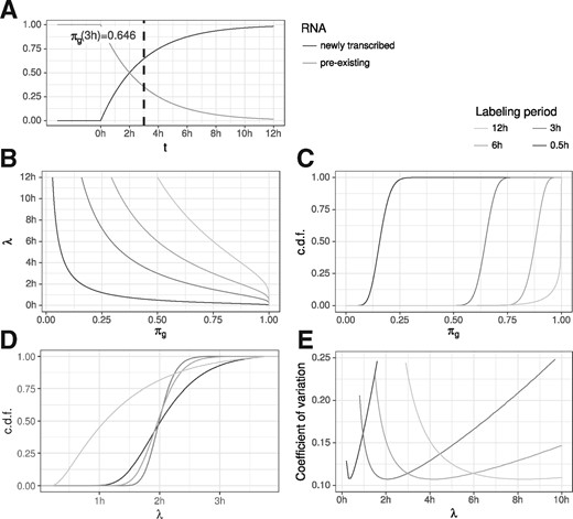
RNA half-life (A) The proportion of new and old RNA of a gene g at any time t, ${\pi }_g(t)$⁠, is directly related to its RNA half-life (here, 2h). (B) The functions are shown that transform the proportion π_g to the RNA half-life for different periods of labeling (see common legend of sub-figures B to E at top right corner). (C) Posterior distributions of a theoretical gene g with 1000 reads and an RNA half-life of 2h for the four different periods of labeling. (D) These posterior distributions for π_g translate to specific posterior distributions on λ, with the one for $t=3h$ being the most precise one. (E) Coefficients of variation (SD divided by the mean) of the posterior distributions on λ for theoretical genes with RNA half-lives between 0 and 10h

To analyze the variance in estimating RNA half-lives using GRAND-SLAM, we first theoretically considered an experiment with typical parameters as observed in the datasets of Herzog et al. (2017), and a gene g with 1000 reads with a half-life of ${\lambda }_g=2h$⁠. For different labeling periods, this gives rise to specific posterior distributions on the proportion parameter π_g (Fig. 5C) which can be transformed into posterior distributions on the estimated RNA half-life (Fig. 5D). Interestingly, the estimate due to 3 h labeling is the most precise, followed by 6h, 0.5 h and 12h. We expanded this analysis to genes with different RNA half-lives, and computed the coefficient of variation (CV) of the posterior distribution of the estimated half-lives (Fig. 5E). The CV is the SD divided by the mean and therefore describes the expected relative deviation. The CV varied greatly depending on the labeling period, with short labeling periods generally most precise for genes with short RNA half-life. In addition, each labeling period has a range of true RNA half-lives where it is most precise and it extremely imprecise for too long or short-lived genes. For example, with 3 h labeling, estimation precision deteriorates for genes with a half-life below half an hour or longer than 8 h. Thus, to precisely estimate the whole range of RNA half-lives in an experiment, several samples with different labeling periods are necessary as well as a method that automatically weighs the contributions of each sample to the overall estimate based on the varying variances. This can be achieved by MAP estimation of the RNA decay rate (Methods Section for details).

4.6 RNA half-lives for mESCs

Herzog et al. (2017) estimated RNA half-lives by pulse-chase experiments: To achieve sufficient labeling, cells were supplied with 4sU for 24 h. After that 4sU was washed out and the drop of conversions was monitored for several time points via SLAM-seq. RNA half-lives were then estimated by fitting an exponential decay model using least squares. These experiment are relatively laborious and introduce the wash-out efficiency as an additional source for potential bias. Furthermore, the least squares fitting does not respect the varying precision of estimating different half-lives with different labeling periods. For comparison, RNA half-lives were also determined using actinomycin D (ActD) treatment and monitoring the drop of RNA levels over time using RNA-seq.

In addition to the pulse-chase and ActD estimates, we used the 3 h or 12 h labeling data or their combination to estimate RNA half-lives for mESCs using our MAP approach (⁠${\text{MAP}}_3,{\text{MAP}}_{12}{,\text{MAP}}_{\text{comb}}$⁠). The correlation coefficients computed over all genes also utilized for comparison in Herzog et al. (2017) showed that MAP_comb performed equally well (⁠$R\approx 0.7$⁠) as the pulse-chase experiments in reproducing the ActD estimates (Fig. 6A). MAP₃ resulted in a similarly high correlation but the MAP₁₂ estimates showed worse correlation (⁠$R\approx 0.46$⁠). For genes with ultra-short (⁠$<2h$⁠) and short (⁠$<3h$⁠) RNA half-lives however, the correlation of the pulse-chase experiment was poor (⁠$R\approx 0$ and $R\approx 0.26$⁠, respectively) and significantly better for MAP₃ and MAP_comb (R > 0.59 and R > 0.49). For genes with longer RNA half-lives, correlations were generally poor, but MAP₁₂ provided the highest correlations (Fig. 6D).

Fig. 6.

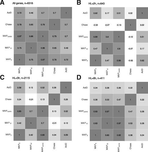
Pearson’s correlation coefficient for RNA half-lifes (A) For n = 6.316 genes, the correlation between any pair of methods estimating RNA half-lives was computed. MAP₃, MAP₁₂ and MAP_comb are the maximum a posterior estimators of GRAND-SLAM computed on the 3h, 12h samples or both. Chase is the exponential decay model fit of Herzog et al. (2017) on the pulse-chase experiments. ActD is the exponential decay model fit for the ActD experiment. (B–D) Correlation coefficients for different sub-sets of genes split according to ultra-short RNA half-life, short RNA half-life and long RNA half-life

Furthermore, MAP_comb always resulted in correlation coefficients (computed for the comparison to the pulse-chase or the ActD experiment) that were close to the better of MAP₃ or MAP₁₂. This indicates that the MAP estimation of the RNA half-live effectively weighs the different precisions obtained for measuring with different labeling periods.

4.7 Differential analysis of RNA half-life changes

Several factors are known to affect the stability of specific RNAs. Most prominently, microRNAs are small RNAs expressed by virtually all eukaryotic cells, that (imperfectly) basepair to cognate sites in mRNAs. Thereby, they guide the RNA induced silencing complex to target mRNAs, which leads to translational repression and induces RNA decay (Bartel, 2009; Jonas and Izaurralde, 2015). By knocking-out Exportin-5 (Xpo5), an essential factor in the biogenesis of the most abundant family of microRNAs in mESCs (miR-291a), repression of mRNA targets of this family is reduced, effectively prolongating their RNA half-life.

In Herzog et al. (2017), this has been analyzed by considering the relative RNA stability computed by comparing the (no4sU corrected) T to C mismatch rates for wild-type (wt) and Xpo5 knock-out (ko) cells. This indeed revealed different sets of predicted microRNA targets to have increased RNA stabilities (Fig. 7A). Using GRAND-SLAM we were able to compute RNA half-lives for both conditions (wt and ko) and compute their log₂ fold changes (Fig. 7B). Comparing the distributions of RNA stabilities with RNA half-live log₂ fold changes already indicates that the latter is a better measure to capture the action of the microRNAs. Indeed, receiver operating characteristic (ROC) analysis revealed RNA half-life log₂ fold change to better agree with predicted microRNA targets than relative RNA stability. However, the overall difference between genes predicted to be a microRNA target and the remaining genes is generally poor, presumably due to secondary effects of knocking down Xpo5 or the difficulty in predicting microRNA targets (Ritchie et al., 2009).

Fig. 7.

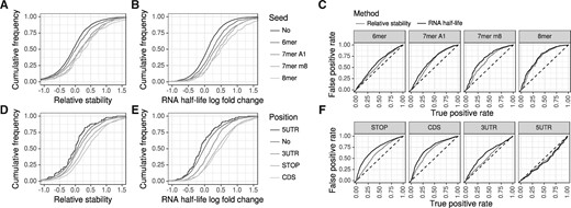
Differential analysis (A and B) We repeated the microRNA target prediction analysis of Herzog et al. (2017). Relative stability values (A) are computed from the corrected conversion counts from the 3h and 12h experiments, RNA half-life log₂ fold changes using GRAND-SLAM (B). The RNA half-lives show a stronger enrichment of targets upon Xpo5 knock-out for all seed types. (C) We performed ROC analyses by treating predicted microRNA targets as the true objects, and mRNAs without seed as the false objects. Then, either the relative stability or RNA half-life log₂ fold change was taken as prediction score. MicroRNA target predictions agreed better with RNA half-lives than with relative stabilities for all four seed types. (D–F) We repeated the m6A modification analyses from Herzog et al. (2017). As expected, no enrichment upon Mettl3 knock-out was found for mRNAs with m6A in the 5’ UTR. For all other mRNA locations defined in Batista et al. (2014), the RNA half-lives show a substantially stronger enrichment of m6A containing mRNAs

Another cellular mechanism affecting RNA stability is N⁶ adenosine methylation (m6A; Meyer and Jaffrey, 2014; Yue et al., 2015). It has been shown that m6A at specific mRNA locations induces mRNA degradation (Wang et al., 2014). m6A modification is performed by the protein complex N6-adenosine-methyltransferase. Thus, by knocking out its 70 kDa sub-unit (Mettl3), genes affected by m6A mediated degradation that have been experimentally determined in mESCs (Batista et al., 2014) are de-repressed. Similarly to the microRNA analyses, relative RNA stabilities can reveal this (Fig. 7A), but RNA half-lives computed by GRAND-SLAM reveal substantially more differences between targets and non-targets (Fig. 7B and C).

5 Discussion

The most successful experimental technique to discriminate between newly transcribed and old RNA is based on metabolic labeling of RNA. To this end, non-toxic nucleoside analogs are introduced into living cells, which are then readily incorporated into newly transcribed RNAs. Previously, total RNA was separated into labeled (newly transcribed) and unlabeled (old) RNA prior to analysis (Dölken et al., 2008; Rabani et al., 2014). The novel approach published recently (Herzog et al., 2017; Riml et al., 2017; Schofield et al., 2018) replaced this biochemical separation with a bioinformatic separation: Nucleoside analogs are chemically converted into distinct nucleoside types and therefore in principle distinguishable based on observed mismatches. However, with incorporation rates of ∼2%, the discrimination between labeled and unlabeled RNA is highly challenging.

Here, we presented a statistical method to precisely estimate the proportion of new and old RNA in such experiments. This is based on a binomial mixture model, where the number of observed, experiment-specific mismatches is generated from one of two binomial distributions for reads from labeled and unlabeled RNA molecules. The output of our method is the full posterior distribution of the proportion of new and old RNA. This posterior is narrow for genes with many reads and for experiments with high incorporation and low sequencing error rates. Thus, it provides a straight-forward mean for quality control.

In addition to sufficient incorporation rates that must be achieved, additional considerations for planning such experiments are important: Herzog et al. (2017) used single-end sequencing with read length 50 bp on a Illumina HiSeq 2500. Longer reads are generally preferrable, as the probability of catching a modified nucleotide increases with longer reads.

Furthermore, paired-end sequencing would provide two significant advantages over single-end reads: First, error rates can be estimated from the other read, since 4sU converted to cytosine results in a T to C mismatch in the first read, and in an A to G mismatch in the second read. Second, especially if RNA is strongly fragmented, read pairs overlap. All nucleotides in the overlapping part are sequenced twice, making the differentiation of true conversions from sequencing errors much easier: The probability for two independent sequencing errors of the same nucleotide is negligibly small. Thus, in such situations, it is possible to decide with almost certainty that a read pair originated from a newly transcribed RNA molecule.

The estimation of sample specific error rates is a crucial component of our method. Here, this has been solved by the observation that error rates were correlated, which we could exploit by a linear regression model. The model was trained on available samples that have not been treated with 4sU, and could predict T to C error rates with sufficient accurracy. A potent alternative would be to use RNA spike-ins such as the ERCC mix (Jiang et al., 2011) in each sample. This way, error rates could be directly estimated by counting mismatches on the ERCC RNAs.

We have shown that the estimated proportions of new and old RNA can be used to compute precise RNA half-lives. Importantly, this (and all other estimates of RNA half-life based on metabolic labeling) heavily relies on the incorporation rate of the nucleoside analog to be constant over time. Considering that they have to cross cell membranes, the cytoplasm and the nuclear membrane to increase their concentration in the nucleus, we expect this assumption to be problematic. 4sU needs time to accumulate, and methods are needed to measure this effectively reduced time of labeling to be considered in estimating RNA half-lives.

We uncovered that using SLAM-seq, short half-lives can be resolved more precisely with short periods of labeling. For such it is difficult to achieve enough 4sU incorporation for our method to estimate the conversion rate. Thus, labeling periods and 4sU concentrations should be carefully tested, potentially in a cell type specific manner.

6 Conclusion

SLAM-seq experiments provide an exciting new technique to access newly transcribed RNA for obtaining RNA half-lives or investigating fast and complex regulatory processes. However, tailored computational analyses approaches for such high-throughput experiments are an essential factor for the success of any study emplyoing SLAM-seq. Here, we provide the first statistical method that is able to precisely delineate the quantities of newly transcribed RNA for each gene and discriminate it from pre-existing RNA before labeling.

Conflict of Interest: F.E. and L.D. declare competing financial interest. A patent application related to this work has been filed.

Acknowledgements

The Helmholtz Institute for RNA-based Infection Research (HIRI) partially supported this work with a seed grant through funds from the Bavarian Ministry of Economic Affairs and Media, Energy and Technology (Grant allocation nos. 0703/68674/5/2017 and 0703/89374/3/2017). L.D. was supported by the European Research Council (grant ERC-2016-CoG 721016HERPES).