Bayesian networks for mass spectrometric metabolite identification via molecular fingerprints

Abstract

Motivation

Metabolites, small molecules that are involved in cellular reactions, provide a direct functional signature of cellular state. Untargeted metabolomics experiments usually rely on tandem mass spectrometry to identify the thousands of compounds in a biological sample. Recently, we presented CSI:FingerID for searching in molecular structure databases using tandem mass spectrometry data. CSI:FingerID predicts a molecular fingerprint that encodes the structure of the query compound, then uses this to search a molecular structure database such as PubChem. Scoring of the predicted query fingerprint and deterministic target fingerprints is carried out assuming independence between the molecular properties constituting the fingerprint.

Results

We present a scoring that takes into account dependencies between molecular properties. As before, we predict posterior probabilities of molecular properties using machine learning. Dependencies between molecular properties are modeled as a Bayesian tree network; the tree structure is estimated on the fly from the instance data. For each edge, we also estimate the expected covariance between the two random variables. For fixed marginal probabilities, we then estimate conditional probabilities using the known covariance. Now, the corrected posterior probability of each candidate can be computed, and candidates are ranked by this score. Modeling dependencies improves identification rates of CSI:FingerID by 2.85 percentage points.

Availability and implementation

The new scoring Bayesian (fixed tree) is integrated into SIRIUS 4.0 (https://bio.informatik.uni-jena.de/software/sirius/).

1 Introduction

Liquid chromatography mass spectrometry (LC-MS) is one of the predominant experimental platforms for the characterization of small molecules in metabolomics and natural products research, and can detect thousands of small molecules simultaneously from a biological sample. Metabolomics, in turn, has been termed ‘apogee of the omics trilogy’ (Patti et al., 2012), as metabolites can serve as a direct signature of biochemical activity. To identify a compound, tandem mass spectrometry is utilized, where a particular molecule is isolated, fragmented by collision with a noble gas or nitrogen, and masses of its fragments are recorded. Until recently, interpretation of corresponding tandem MS spectra was mainly limited to searching in spectral libraries of reference compounds. Unfortunately, spectral libraries are vastly incomplete, containing spectra from less than 20 000 small molecules (Vinaixa et al., 2016); in comparison, the molecular structure database PubChem holds more than 100 million entries (Kim et al., 2016). This gap will presumably further widen in the future, as ‘low-hanging fruit’ (commercial standards) have already been added to spectral libraries. To this end, a large fraction of the compounds in a metabolomics LC-MS run remain unidentified; depending on the organism, this can be the case for up to 98% of the compounds (da Silva et al., 2015). Hence, it is not surprising that ‘compound identification’ is consistently named as one of the biggest challenges in MS-based metabolomics.

Starting in 2008 (Hill et al., 2008), methods have been developed to search tandem MS data in molecular structure databases (Allen et al., 2015, 2016; Heinonen et al., 2012; Ridder et al., 2013; Ruttkies et al., 2016; Shen et al., 2014; Tsugawa et al., 2016; Verdegem et al., 2016; Wang et al., 2014), see Hufsky et al. (2014) and Hufsky and Böcker (2017) for reviews. It must be understood that small molecule identification via tandem MS is a much more challenging problem than, say, peptide identification. At present, CSI:FingerID (Dührkop et al., 2015) and its Input Output Kernel Regression variant (Brouard et al., 2016) are the best-performing methods for this task (Dührkop et al., 2015; Schymanski et al., 2017). CSI:FingerID is frequently used in the scientific community, with more than 700 000 query compounds processed in 2017. CSI:FingerID uses the query’s tandem MS data to estimate a fragmentation tree, then uses machine learning to predict the query’s molecular fingerprint (a binary vector encoding the presence or absence of a fixed set of molecular structures) from fragmentation spectrum and tree. As the last step of the CSI:FingerID pipeline, one compares the predicted query fingerprint with the target fingerprints from the molecular structure database. Dührkop et al. (2015) suggested two statistical scores which perform best in evaluations; both scores implicitly assume independence between molecular properties.

Here, we focus on the last step of the CSI:FingerID pipeline, and present a scoring which no longer assumes independence. We model dependencies between molecular properties using a Bayesian network; to ease calculations, we assume that this network is a tree. Our scoring uses Bayesian networks in a non-standard fashion: The previous step of the CSI:FingerID pipeline estimates the probability of each molecular probability to be present via machine learning; we use these as marginal probabilities of the random variables in the Bayesian network. Second, we estimate the tree topology of the Bayesian network using the mutual information of molecular properties for instance candidates. Third, we estimate ‘desired’ covariances between random variables connected in the tree. Finally, for each edge we estimate joint probabilities that simultaneously satisfy the marginal probability constraints and the estimated covariance values. Now, the joint probability of the complete evidence is used as a score. Our model takes into account both dependencies of molecular properties from deterministic fingerprints, and dependencies from fingerprint prediction: For example, an overly optimistic estimate for one property may result in an overly optimistic estimate for another property. We find that the resulting score performs significantly better than all previous scores.

2 Preliminaries

Elucidation of stereochemistry is currently beyond the power of automated search engines (or even beyond the power of tandem MS), so CSI:FingerID tries to recover the correct constitution of the query molecule: that is, the identity and connectivity of the atoms including bond multiplicities, but no spacial (stereochemistry) information. Here, we refer to the constitution of a molecule as its structure.

We start by describing the basic mechanisms behind fingerprint-based structure search (Dührkop et al., 2015). Molecular fingerprints encode the structure of a molecule: Most commonly, these are binary vectors of fixed length where each bit describes the presence or absence of a particular, fixed molecular property, usually the existence of a certain substructure. Numerous fingerprint types have been proposed during the last years, such as PubChem CACTVS fingerprints (881 molecular properties) or MACCS fingerprints (166 molecular properties). Given the molecular structure of a compound, we can deterministically compute its molecular fingerprint (Willighagen et al., 2017). See Figure 1 for an example. Molecular fingerprints have been extensively used for virtual screening and related tasks. Formally, let $1,\dots ,n$ be the molecular properties; then, a (binary) fingerprint is a vector from ${\{0,1\}}^n$⁠. Each molecular structure has a (not necessarily unique) fingerprint assigned to it. Clearly, molecular properties do not have to be independent; this is particularly the case if the substructure of one molecular property is contained in the substructure of another molecular property (Fig. 1).

Fig. 1.

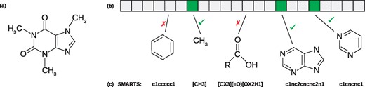
Molecular fingerprint of a molecular structure. From the molecular structure (a) the molecular fingerprint (b) can be deterministically computed. Each position of the fingerprint corresponds to a molecular property specified as SMARTS string (c) and exemplified by a structure matching each SMARTS. The pyrimidine ring property (rightmost illustrated structure) is a substructure of the heterocyclic purine to its left; every structure containing heterocyclic purine must also contain a pyrimidine ring

When searching in a structure database such as PubChem, we first extract a set of molecular structure candidates; this is done using the mass, or one or more molecular formula candidates of the query compound (Dührkop et al., 2015). Each candidate structure is deterministically transformed to a binary candidate fingerprint. The tandem MS data and fragmentation tree of the query compound is used to predict the fingerprint of the query compound, using an array of Support Vector Machines (Dührkop et al., 2015; Heinonen et al., 2012; Shen et al., 2014).

As the last step of CSI:FingerID, we compare the predicted fingerprint with the deterministic, binary candidate fingerprints. Unit scores simply count the number of differences between the predicted fingerprint and each candidate fingerprint. Heinonen et al. (2012) used the accuracy of individual SVMs to weight the scoring, but this does not perform better than unit scoring (Dührkop et al., 2015). Dührkop et al. (2015) suggested and evaluated different scoring variants, and found that two variants consistently outperformed all others in evaluation: Namely, the ‘Platt’ score and the ‘modified Platt’ score.

Both scores use Platt probabilities (Platt, 2000) for fine-grained predictions: Instead of a binary prediction of a SVM, we use a sigmoid function to predict the posterior probability for the presence of the molecular property, with parameter estimated from the training data to predict this probability. Let $\mathcal{D}=(p_1,\dots ,p_n)\in {[0,1]}^n$ be the Platt probability estimates, and let $\mathcal{M}=(x_1,\dots ,x_n)\in {\{0,1\}}^n$ be a candidate fingerprint; assuming independence between all molecular property pairs, we can estimate the posterior probability of the fingerprint candidate $\mathcal{M}$ as

$$\mathbb{P}\left(\mathcal{M}\right|\mathcal{D})=\prod _{i=1,\dots ,n}\{\begin{array}{ll}{p}_i\hfill & \text{if} x_i=1,\hfill \\ 1-p_i\hfill & \text{if} x_i=0.\hfill \end{array}$$

(1)

This has been referred to as ‘Platt score’ in (Dührkop et al., 2015); maximizing this score corresponds to a Maximum A Posteriori Estimator, and results in about 3.5 percentage points more correct identifications than unit scores. In contrast, the ‘modified Platt’ score from (Dührkop et al., 2015) was found by trial and error, combines Platt probabilities and sensitivity/specificity estimates of the binary predictors in a counterintuitive fashion: Namely,

$$\begin{array}{l}\prod _{i=1}^n\{\begin{array}{ll}{p}_i^{0.75}·{(1-sen{s}_i)}^{0.25}\hfill & \text{if} p_i\ge 0.5 \text{and} x_i=1\hfill \\ {(1-p_i)}^{0.75}\hfill & \text{if} p_i\ge 0.5 \text{and} x_i=0\hfill \\ p_i^{0.75}\hfill & \text{if} p_i<0.5 \text{and} x_i=1\hfill \\ {(1-p_i)}^{0.75}·{(1-spe{c}_i)}^{0.25}\hfill & \text{if} p_i<0.5 \text{and} x_i=0\hfill \end{array}\hfill \end{array}$$

(2)

where $sen{s}_i$ is the sensitivity and $spe{c}_i$ the specificity of the ith binary predictor. While this score has no statistical interpretation, modified Platt (2) consistently outperforms the Platt score (1) by a margin of about 1.5 percentage points.

3 Tree-based posterior probability estimation

For the presentation of our method, we rewrite (1) using binary random variables: Assume that X_i is a binary random variable such that $\mathbb{P}(X_i=1)=p_i$⁠. Then, $\mathbb{P}(X=x)$ with $X=(X_1,\dots ,X_n)$ is the posterior probability of the model $x:=\mathcal{M}$⁠; and $\mathbb{P}(X=x)=\prod _i\mathbb{P}(X_i=x_i)$ if all random variables are independent.

We want to modify the posterior probability estimate to take into account dependencies between molecular properties. We model dependencies between random variables X_i, X_j (molecular properties i, j) as a rooted tree$T=(V,E)$ with $V=\{1,\dots ,n\}$ and $E\subseteq V\times V$⁠, such that edges $(i,j)\in E$ describe conditional dependencies between random variables X_i and X_j; this is the simplest case of a Bayesian network. Let r be the root of T; all edges in T point away from r, which is also called ‘arborescence’. Then, the joint distribution can be written as

$$\begin{array}{l}\mathbb{P}(X_1,\dots ,X_n)=\mathbb{P}\left(X_r\right)·\prod _{(i,j)\in E}\mathbb{P}\left(X_j\right|X_i)\hfill \\ =\mathbb{P}\left(X_r\right)·\prod _{(i,j)\in E}\frac{\mathbb{P}(X_i,X_j)}{\mathbb{P}\left(X_i\right)}\hfill \end{array}$$

(3)

where $\mathbb{P}(X_i,X_j)$ is the joint distribution of X_i and X_j. In Bayesian network analysis, relationships between adjacent nodes would usually be specified via conditional probability tables for $\mathbb{P}\left(X_j\right|X_i)$⁠. But for the problem at hand, we cannot estimate these conditional probabilities directly; to this end, we use the indirect estimation procedure via the joint distribution $\mathbb{P}(X_i,X_j)$⁠.

How do we estimate $\mathbb{P}(X_i=x_i,X_j=x_j)$? We know the marginal probabilities $\mathbb{P}(X_i=1)=p_i$ and $\mathbb{P}(X_j=1)=p_j$ (Platt estimates of posterior probabilities) from the data $\mathcal{D}$⁠. As X_i and X_j are binary, we have to consider exactly four cases: Set $q_{11}:=\mathbb{P}(X_i=1,X_j=1),q_{10}:=\mathbb{P}(X_i=1,X_j=0),\hspace{0.17em}{q}_{01}:=\mathbb{P}(X_i=0,X_j=1)$ and $q_{00}:=\mathbb{P}(X_i=0,X_j=0)$⁠. As the marginal probabilities are known, $q_{11}+q_{10}=p_i$ and $q_{11}+q_{01}=p_j$ must hold. We also know $q_{11}+q_{10}+q_{01}+q_{00}=1$⁠. This means that we have one degree of freedom for choosing $q_{11},q_{10},q_{01},q_{00}$⁠.

We decided to use this degree of freedom, to ensure that the covariance of X_i, X_j equals some predetermined value $co{v}_{i,j}\in ℝ$⁠. This models our observation that certain molecular properties are correlated. The covariance of the binary random variables X_i, X_j is

$$\text{cov}(X_i,X_j)=\mathbb{E}\left(X_i{X}_j\right)-\mathbb{E}\left(X_i\right)\mathbb{E}\left(X_j\right)=q_{11}-p_i{p}_j,$$

since clearly $\mathbb{E}\left(X_i\right)=p_i$ and $\mathbb{E}\left(X_j\right)=p_j$⁠. In total, we have reached four linear equations for the four unknowns $q_{11},q_{10},q_{01},q_{00}$⁠, namely:

$$\begin{array}{l}{q}_{11}+q_{10}=p_i,\hspace{1em}{q}_{11}+q_{01}=p_j,\hfill \\ q_{11}+q_{10}+q_{01}+q_{00}=1\hfill \end{array}$$

(4)

$$q_{11}=co{v}_{i,j}+p_i{p}_j$$

(5)

Unfortunately, solving (4) and (5) may result in a solution that does not satisfy the obvious requirement $q_{11},q_{10},q_{01},q_{00}\in [0,1]$⁠. Whereas we think of Equation (4) as inevitable requirements, (5) is a somewhat more subjective choice; to this end, we modify (5) accordingly:

$$q_{11}=\max \{0,p_i+p_j-1,\min \{p_i,p_j,co{v}_{i,j}+p_i{p}_j\left\}\right\}$$

(6)

It is straightforward but cumbersome to check that choosing $q_{11},q_{10},q_{01},q_{00}$ according to (4) and (6) does indeed satisfy $q_{11},q_{10},q_{01},q_{00}\in [0,1]$⁠, and that the established bounds are tight: For example, choosing $q_{11}<p_i+p_j-1$ will violate $q_{00}\ge 0$⁠. The covariance $\text{cov}(X_i,X_j)$ of the resulting random variables does not necessarily equal $co{v}_{i,j}$⁠, but if not, it is chosen ‘as large’ or ‘as small’ as possible. See the Lemmas below for details.

We can now determine joint probabilities $\mathbb{P}(X_i=x_i,X_j=x_j)$ for every edge (i, j), and use (3) to estimate the probability of evidence X = x, that is, the joint probability $\mathbb{P}(X_1=x_1,\dots ,X_n=x_n)$⁠; we use this estimate as the new score. To avoid numerical instabilities, we apply Laplace (additive) smoothing to probabilities $\mathbb{P}\left(X_i\right)$ and $\mathbb{P}(X_i,X_j)$ when computing (3). Computing $\mathbb{P}(X_i=x_i,X_j=x_j)$ can be carried out in constant time, so computing $\mathbb{P}(X=x)$ requires O(n) time.

We now give formal proofs that choosing $q_{11},q_{10},q_{01},q_{00}$ as described above results in probabilities from $[0,1]$ (Lemma 1); and that choosing a larger (Lemma 2) or smaller q₁₁ (Lemma 3) is not possible in case we deviate from the target value $co{v}_{i,j}+p_i{p}_j$⁠.

 

Lemma 1. Given$p_i,p_j\in [0,1]$and$co{v}_{i,j}\in ℝ$. Then, $q_{11}:=\max \{0,p_i+p_j-1,\min \{p_i,p_j,co{v}_{i,j}+p_i{p}_j\left\}\right\}$from (6), $q_{10}:=p_i-q_{11},q_{01}:=p_j-q_{11}$and$q_{00}:=1-(q_{11}+q_{10}+q_{01})$all satisfy$q_{11},q_{10},q_{01},q_{00}\in [0,1]$⁠.

Proof. Assume $q_{11},q_{10},q_{01},q_{00}$ have been chosen as described. We first infer $q_{11}\le \max \{p_i+p_j-1,p_i\}\le \max \{p_i,p_i\}=p_i$⁠, and analogously $q_{11}\le \max \{p_i+p_j-1,p_j\}\le p_j$⁠. This implies $q_{11}\in [0,1]$ as $q_{11}\ge 0$ is clear, and $q_{11}\le p_i\le 1$⁠. Now, $q_{11}\le p_i$ implies $q_{10}=p_i-q_{11}\ge p_i-p_i=0$⁠, and $q_{11}\le p_j$ implies $q_{01}=p_j-q_{11}\ge p_j-p_j=0$⁠. Furthermore, $q_{11}\ge p_i+p_j-1$ implies $q_{10}=p_i-q_{11}\le p_i-(p_i+p_j-1)=1-p_j\le 1$ and $q_{01}=p_j-q_{11}\le 1-p_i\le 1$⁠. Hence, we have established $q_{10},q_{01}\in [0,1]$⁠. Finally, $q_{11}\ge p_i+p_j-1$ implies $q_{11}+q_{10}+q_{01}=p_i+p_j-q_{11}\le p_i+p_j-(p_i+p_j-1)=1$ and, hence, $q_{00}\ge 0$⁠. With $q_{00}=1-(q_{11}+q_{10}+q_{01})\le 1$ we infer $q_{00}\in [0,1]$⁠.              □

 

Lemma 2. Given$p_i,p_j\in [0,1],\hspace{0.17em}co{v}_{i,j}\in ℝ$, and q₁₁ from (6) such that$q_{11}<co{v}_{i,j}+p_i{p}_j$. Then, any${\overline{q}}_{11}>q_{11}$with${\overline{q}}_{10}:=p_i-{\overline{q}}_{11}$⁠, ${\overline{q}}_{01}:=p_j-{\overline{q}}_{11}$and${\overline{q}}_{00}:=1-({\overline{q}}_{11}+{\overline{q}}_{10}+{\overline{q}}_{01})$cannot simultaneously satisfy${\overline{q}}_{11},{\overline{q}}_{10},{\overline{q}}_{01},{\overline{q}}_{00}\in [0,1]$⁠.

Proof. We do a case distinction, based on the maximum calculation of q₁₁: (i) If $q_{11}=0$ then $p_i,p_j\ge 0$ implies $co{v}_{i,j}+p_i{p}_j\le 0=q_{11}$⁠, in contradiction to our assumptions. (ii) If $q_{11}=p_i+p_j-1$ then $q_{11}<co{v}_{i,j}+p_i{p}_j$ implies $\min \{p_i,p_j\}\le p_i+p_j-1$⁠. Assume w.l.o.g. that $p_i\le p_j$⁠, then $p_i\le p_i+p_j-1$ and, hence, p_j = 1. We infer ${\overline{q}}_{11}>q_{11}=p_i+p_j-1=p_i$ and, hence, ${\overline{q}}_{10}=p_i-{\overline{q}}_{11}<0$⁠. (iii) If $q_{11}=\min \{p_i,p_j,co{v}_{i,j}+p_i{p}_j\}$ then $q_{11}=\min \{p_i,p_j\}<co{v}_{i,j}+p_i{p}_j$⁠. Hence, ${\overline{q}}_{11}>\min \{p_i,p_j\}$⁠, and either ${\overline{q}}_{10}=p_i-{\overline{q}}_{11}<0$ or ${\overline{q}}_{01}=p_j-{\overline{q}}_{11}<0$ must hold.    □

 

Lemma 3. Given$p_i,p_j\in [0,1],\hspace{0.17em}co{v}_{i,j}\in ℝ$, and q₁₁ from (6) such that$q_{11}>co{v}_{i,j}+p_i{p}_j$. Then, any${\overline{q}}_{11}<q_{11}$with${\overline{q}}_{10}:=p_i-{\overline{q}}_{11}$⁠, ${\overline{q}}_{01}:=p_j-{\overline{q}}_{11}$and${\overline{q}}_{00}:=1-({\overline{q}}_{11}+{\overline{q}}_{10}+{\overline{q}}_{01})$cannot simultaneously satisfy${\overline{q}}_{11},{\overline{q}}_{10},{\overline{q}}_{01},{\overline{q}}_{00}\in [0,1]$⁠.

Proof. We again do a case distinction: (i) If $q_{11}=0$ then ${\overline{q}}_{11}<0$⁠. (ii) If $q_{11}=p_i+p_j-1$ then ${\overline{q}}_{11}<p_i+p_j-1$ and, hence, ${\overline{q}}_{11}+{\overline{q}}_{10}+{\overline{q}}_{01}=p_i+p_j-{\overline{q}}_{11}>p_i+p_j-(p_i+p_j-1)=1$⁠, so ${\overline{q}}_{00}<0$⁠. (iii) If $q_{11}=\min \{p_i,p_j,co{v}_{i,j}+p_i{p}_j\}$ then $q_{11}\le co{v}_{i,j}+p_i{p}_j$ in contradiction to our assumptions.            □

4 Finding the tree and estimating covariances

It must be understood that in principle, every tree can be used for our computations, and there are no ‘incorrect’ trees; our obvious goal is to reach an improved identification rate. In view of the superexponential number of trees with n nodes, we restrict our evaluation to trees that ‘turn up naturally’ from the data. We show how to estimate the tree structure, and the desired covariance values for every edge of the tree. The tree structure is estimated solely from molecular structure data; for covariance estimation, we take into account the training data and, in particular, dependencies between predictions between molecular properties. We distinguish two cases: In the first case, we estimate one ‘global’ fixed tree structure and desired covariance values, which is then used to score candidates for any query. In the second case, we take into account that for each query, only candidates with a particular molecular formula are considered. We compute an individual tree for this molecular formula, and also consider the molecular formula when estimating covariances. Note that molecular structure candidates of the same molecular formula are also structurally similar. As a consequence, molecular properties can be non-informative, as all structure candidates either do or do not have the property. Computing individual trees prevents that non-informative properties can ‘block’ the path between informative properties in the Bayesian scoring tree: Non-informative properties will have mutual information zero, and will be inserted as leaves in the individual tree.

4.1 Fixed tree structure

To prevent overfitting, we do not search for a tree that maximizes identification rates. Instead, we estimate the tree structure using all molecular structures from some structure database. Mutual information is a natural choice to measure how much information we gain from one molecular property about another molecular property. We use mutual information between molecular properties from a molecular structure database as a proxy for the interdependence between random variables (predictions). For each structure in the database, we (deterministically) compute the corresponding molecular fingerprint, resulting in a multiset $\mathcal{F}$ of fingerprints. For any two molecular properties i, j we consider the corresponding binary random variables I, J; estimation of (joint) probabilities for I, J is straightforward by counting in $\mathcal{F}$⁠. We then compute the mutual information between I and J, quantifying the ‘amount of information’ obtained about I through J. This results in a complete graph G with nodes $\{1,\dots ,n\}$⁠, where every pair of nodes (molecular properties) is connected by an edge with weight equal to the mutual information. The tree structure is computed as a maximum spanning tree in this graph, in $O\left(\right|V{|}^2·\hspace{0.17em}\text{log}\hspace{0.17em}\left|V\right|)$ time using Prim’s algorithm (with a binary heap) or Kruskal’s algorithm. Finally, we arbitrarily root this tree, as the choice of the root does not influence our computations. Some edges of the tree may have weight (mutual information) zero; this is an artifact of computing a spanning tree which connects all nodes.

Let $T=(V,E)$ be the tree; we now estimate desired covariance values. Here, we consider all compounds in the training data; only for these, we can estimate if wrong predictions of one molecular property, result in wrong predictions of another property. Each compound from the training data consists of a true fingerprint $(y_1,\dots ,y_n)\in {\{0,1\}}^n$ and a predicted (Platt) fingerprint $(p_1,\dots ,p_n)\in {[0,1]}^n$⁠.

Consider edge $(i,j)\in E$ from molecular property i to j. We partition compounds from the training data into four batches (0, 0), (0, 1), (1, 0) and (1, 1), such that a training compound with true fingerprint $(y_1,\dots ,y_n)$ is sorted into batch $(y_i,y_j)\in {\{0,1\}}^2$⁠:

$${\mathcal{P}}_{i,j}^{(s,t)}:=\left\{\right(p_i,p_j)\hspace{0.17em}:\hspace{0.17em}(y_i,y_j)=(s,t\left)\right\}$$

We compute four covariance estimates $co{v}_{i,j}^{(s,t)}$⁠, one for each batch ${\mathcal{P}}_{i,j}^{(s,t)}$ with $(s,t)\in {\{0,1\}}^2$⁠. Set $\mathcal{P}:={\mathcal{P}}_{i,j}^{(s,t)}$ for brevity; these are our observations used to estimate the covariance. To avoid empty batches and prevent overfitting, we add four pseudo-observations (0, 0), (0, 1), (1, 0) and (1, 1) to the observations $\mathcal{P}$⁠. We again interpret Platt probabilities p_i as the probability that a binary random variable X_i satisfies X_i = 1. The normalized number of observations $\mathcal{N}[a,b]\in (0,1)$ for $a,b\in \{0,1\}$ is

$$\begin{array}{ll}\mathcal{N}[1,1]\hfill & =\frac{1}{\left|\mathcal{P}\right|}·{\sum }_{(p,p\prime )\in \mathcal{P}}pp\prime ,\hfill \\ \dots \hfill & \hfill \\ \mathcal{N}[0,0]\hfill & =\frac{1}{\left|\mathcal{P}\right|}·{\sum }_{(p,p\prime )\in \mathcal{P}}(1-p)(1-p\prime )\hfill \end{array}$$

(7)

We then estimate the desired covariance as

$$co{v}_{i,j}^{(s,t)}:=\mathcal{N}[1,1]-\left(\mathcal{N}\right[1,1]+\mathcal{N}[1,0\left]\right)·\left(\mathcal{N}\right[1,1]+\mathcal{N}[0,1\left]\right).$$

Given a candidate fingerprint $(x_1,\dots ,x_n)\in {\{0,1\}}^n$⁠, we want to compute its joint probability $\mathbb{P}(X_1=x_1,\dots ,X_n=x_n)$ according to (3). For every edge $(i,j)\in E$⁠, we set $co{v}_{i,j}=co{v}_{i,j}^{(s,t)}$ for $s:=x_i$ and $t:=x_j$⁠, and proceed to estimate $\mathbb{P}(X_i,X_j)$ as described in the previous section. Hence, every candidate fingerprint has individual covariance estimates; in the previous section, we omitted this technical detail for the sake of readability.

Finally, for artifact edges with mutual information zero, we also assume covariance $co{v}_{i,j}^{(s,t)}=0$⁠.

4.2 Individual trees

Next, we want to compute the tree and desired covariances for each query individually. Regarding the tree, we use all fingerprints from PubChem that have the molecular formula of the query when computing the mutual information. For the covariance, we proceed as described above, but again only consider those compounds from the training data that have the molecular formula of the query. But there are potentially only few such training compounds, so the method is prone to overfitting. We use the following two modifications to overcome this issue: First, when estimating the observation matrix for the query molecular formula, we add the normalized observation matrix (7) estimated from all training data as ‘pseudocounts’. We give this global ‘pseudocounts’ a weight of 14 if there are at least 10 global observations (and the 4 pseudo instances); for fewer global observations, we use the number of global observations (plus pseudo instances) as weight. Second, we do not only use compounds from the training data with identical molecular formula as the query; instead, we allow that training compound and query molecular formula differ by some biotransformation, such as the addition of a water H₂O.

5 Data

Next to spectra from MassBank (Horai et al., 2010) and GNPS (Wang et al., 2016) we trained CSI:FingerID on data from the NIST 2017 database (National Institute of Standards and Technology, v17). As evaluated here, CSI:FingerID 1.12 is trained is trained on 13 766 structures and 16 865 measurements in positive ion mode. For one compound, a library may contain several tandem MS spectra, which are merged by SIRIUS 3.6 into a single spectrum (Böcker and Dührkop, 2016). As described in previous publications (Böcker and Dührkop, 2016; Dührkop et al., 2015, 2018), we discard certain instances based on strong deviation of the precursor mass etc.; we leave out the tedious details, as these are not important here. As an independent dataset, we use the commercial ‘MassHunter Forensics/Toxicology PCDL’ library (Agilent Technologies, Inc.) with 3451 spectra.

Tree structures are computed from molecular structures, without taking into account tandem MS data. To compute the fixed tree structure we use 236 656 molecular structures from databases of biological interest, namely KNApSAcK (Shinbo et al., 2006), HMDB (Wishart et al., 2012), ChEBI (Hastings et al., 2012), KEGG (Kanehisa et al., 2016), BioCyc (Caspi et al., 2014), UNPD (Gu et al., 2013) and MeSH-annotated compounds from PubChem (Kim et al., 2016). In contrast, the individual tree structures specific for one query are computed from all PubChem structures with the same molecular formula (or the molecular formula plus corresponding biotransformation). We use a local copy of PubChem from August 13, 2017 containing 93 859 798 compounds and 73 444 774 structures.

6 Results and discussion

CSI:FingerID and its Input Output Kernel Regression variant (Brouard et al., 2016) are currently the best-performing methods for searching with tandem MS data in molecular structure databases. This has been demonstrated in two blind competitions, namely the Critical Assessment for Small Molecule Identification (CASMI) contests 2016 and 2017 (http://casmi-contest.org/). CASMI 2016 (category 2) provided data for 127 compounds in positive ion mode, of which CSI:FingerID correctly identified 70 (Schymanski et al., 2017), more than twice the number of the best non-CSI:FingerID method: In detail, MS-FINDER (Tsugawa et al., 2016), CFM-ID (Allen et al., 2015), MAGMA+ (Verdegem et al., 2016) and MetFrag2.3 (Ruttkies et al., 2016; Wolf et al., 2010) had 32, 27, 16 and 15 correct identifications, respectively. In CASMI 2017 (category 4), CSI:FingerID identified sixfold the number of compounds of the best non-CSI: FingerID method. This is in agreement with finding by Dührkop et al. (2015) who found that CSI:FingerID outperforms the runner-up 2.5-fold. To this end, we refrain from evaluating against other methods.

We follow the evaluation setup of Dührkop et al. (2015). In our evaluation, we make sure that all evaluated structures are novel: That is, no tandem MS data from a compound with the same structure is present in the training data. For example, for d-threonine to be novel, the training data must not contain any tandem mass spectra for d-threonine, l-threonine, or (d or l)-allo-threonine. We use 10-fold cross validation when predicting fingerprints for the training data; no two folds contain the same structure. For the independent dataset, we ensure novel structure evaluation by using, for each query, the cross-validation model which does not contain the query structure; in case the query structure is not preset in the training data, we use a model trained on all training data.

We extracted 91 molecular formulas of biotransformations from Rogers et al. (2009) and Li et al. (2013); we excluded large modifications above 100 Da and modifications not composed from CHNO, resulting in 29 modifications used here: namely, C₂H₂, C₂H₂O, C₂H₃NO, C₂H₃O₂, C₂H₄, C₂O₂, C₃H₂O₃, C₃H₅NO, C₃H₅NO₂, C₃H₅O, C₄H₂N₂O, C₄H₃N₃, C₄H₄O₂, C₅H₇, C₅H₇NO, C₅H₉NO, CH₂, CH₂ON, CH₃N₂O, CHO₂, CO, CO₂, H₂, H₂O, N, NH, NH₂, NH₃ and O. These biotransformations are used to increase the number of specific compounds used to compute the covariances for individual trees.

CSI:FingerID reached 31.8% correct identifications in cross-validation on the GNPS dataset (Dührkop et al., 2015), which was 2.6-fold higher than the runner-up method. Since then, numerous methodical improvements (for example, novel kernels) as well as additional training data have further improved the performance of CSI:FingerID. On the other hand, PubChem, the database we search in, has greatly increased in size which, in turn, makes is harder to identify the correct molecular structure. We evaluate on 16 865 cross-validation compounds and the independent dataset from Agilent. For each method, we report the ratio of instances where a method ranked the correct structure in its top k output, for $k=1,\dots ,10$⁠. We evaluate the new scores—termed ‘Bayesian (fixed tree)’, ‘Bayesian (individual tree)’ and ‘Bayesian (biotransformations)’—in addition to the Platt and modified Platt scores from (Dührkop et al., 2015). All new scores are derived from the standard Platt score, which makes it the baseline method. Still, ‘modified Platt’ is the currently best-performing score to beat.

We find that all new scores outperform Platt and modified Platt in cross-validation, see Figure 2 and Table 1. Bayesian (individual tree and biotransformations) achieve highest identification rates of 43.62 and 42.92%, respectively. This is an improvement of 3.20–3.89 percentage points to the baseline, and improves modified Platt by 2.85 percentage points.

Table 1.

Identification rates with standard deviations using different CSI: FingerID scores on 10-fold cross-validation

Method	Top 1	Top 5	Top 10
Bayesian (individual tree)	43.62 ± 1.53	77.67 ± 0.90	85.23 ± 1.05
Bayesian (biotransformations)	42.92 ± 1.52	76.68 ± 0.82	84.39 ± 0.97
Bayesian (fixed tree)	41.51 ± 1.10	74.91 ± 0.88	83.19 ± 1.18
Modified Platt	40.77 ± 0.92	74.91 ± 1.35	83.02 ± 1.35
Platt	39.72 ± 1.44	73.62 ± 1.33	82.19 ± 1.34

Note: We report the percentage where the correct structure was identified in the top k.

Fig. 2.

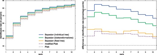
Left: Identification rates using different CSI:FingerID scores, for cross-validation. We report the percentage of instances where the correct structure was identified in the top k, for varying k. Scores are Platt, modified Platt, Bayesian (fixed tree), Bayesian (individual tree) and Bayesian (biotransformations). Note the zoomed y-axis. Right: Percentage point differences in identification rates against the Platt score, for cross-validation

Identification rates on Agilent are all slightly lower than on cross-validation. Bayesian (biotransformations) achieves the best top 1 rate with 39.86% (Fig. 3). Both Bayesian (biotransformations) and Bayesian (individual tree) improve on the modified Platt’s identification rate by more than 1.28 percentage points.

Fig. 3.

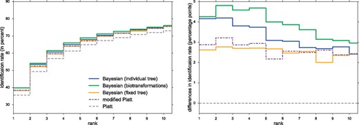
Left: Identification rates using different CSI:FingerID scores, for Agilent. We report the percentage of instances where the correct structure was identified in the top k, for varying k. Scores are Platt, modified Platt, Bayesian (fixed tree), Bayesian (individual tree) and Bayesian (biotransformations). Note the zoomed y-axis. Right: Percentage point differences in identification rates against Platt score, for Agilent

Predicting fingerprints of Agilent compounds, we ensured to use CSI:FingerID models not trained on this specific structure. Nevertheless, we used all cross-validation compounds to compute covariances for the three Bayesian scores. We want to asses how this influences the performance on the Agilent dataset. To this end, we split the dataset in two groups: Agilent (known structure) with 1868 compounds and Agilent (unknown structure) with 1583 compounds. The first group contains those compounds with structure contained in the cross-validation dataset; the second contains completely novel compounds not even used for estimating covariance. See Figure 4: On Agilent with known structure, Bayesian (biotransformations) and Bayesian (individual tree) clearly outperform all other methods. On Agilent with unknown structure, Bayesian (individual tree) loses its performance edge over modified Platt, but still clearly outperforms Platt. Bayesian (biotransformations) consistently outperforms both, Platt and modified Platt, on all datasets, even on completely novel compounds. We stress that all three new scores improve on their baseline method in every case. We argue that all three Bayesian scores only have minor tendencies to overfit, as they still beat their baseline method on novel structures. Actually, Bayesian (biotransformations) generalizes good enough to beat modified Platt on all datasets.

Fig. 4.

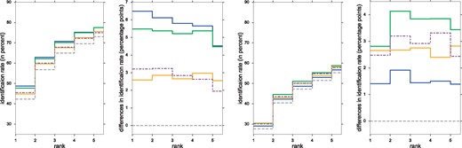
Left: Identification rates and differences using different CSI:FingerID scores, for Agilent (known structures). Right: Identification rates and differences using different CSI:FingerID scores, for Agilent (unknown structures). For legend and further details see Figure 3

Finally, we evaluated the 127 instances in positive ion mode from CASMI 2016 (Schymanski et al., 2017), again ensuring that all structures are novel when predicting fingerprints. All Bayesian scores outperform Platt and modified Platt: Bayesian (biotransformations) and Bayesian (individual tree) reach 36.61%, Bayesian (fixed tree) reaches 35.04% correct identifications. In comparison, Platt and modified Platt identify 26.38 and 30.31% correctly.

Are the reported improvements statistically significant? We evaluated significance using the one-tailed Welch’s t-test for cross validation, and the one-tailed sign test for wins (one method reaches a better rank than the other method) for all datasets. We test Bayesian (biotransformations) against Platt and modified Platt. Against Platt, all P-values are highly significant (below $6.4\times {10}^{-5}$⁠). Against modified Platt, all P-values except for ‘wins on Agilent dataset’ are significant (below 0.0017). See Table 2 for details.

Table 2.

P-values of method comparison for Bayesian (biotransformations) versus Platt and modified Platt

Statistical test	Versus Platt	Versus mod. Platt
Cross validation, Welch’s t-test (ten folds)	$6.4\times {10}^{-5}$	$8.0\times {10}^{-4}$
Cross validation, sign test on wins (⁠$N=16\hspace{0.17em}865$⁠)	$1.5\times {10}^{-60}$	$3.1\times {10}^{-21}$
Agilent, sign test on wins (⁠$N=3\hspace{0.17em}451$⁠)	$2.4\times {10}^{-11}$	0.57
CASMI 2016, sign test on wins (N = 127)	$8.4\times {10}^{-6}$	0.0017

Note: Using a one-tailed Welch’s t-test, we test if variations in correct identifications are significantly larger between methods than between folds. For the one-tailed sign test, a ‘win’ means that method A reaches a better rank than method B; ties for the top rank are removed (no method can outperform the other method for these seamingly simple instances), other ties are equally distributed between the two methods (conservative approach). For Agilent, wins of Bayesian (biotransformations) versus modified Platt, no method performs significantly better than the other.

7 Conclusion

We have introduced a new score for CSI:FingerID that does not only outperform previous scores for searching in molecular structure databases, but also allows for a statistical interpretation. The score interprets the problem as computing the probability of evidence in a Bayesian network. We apply Bayesian networks in a novel and unexpected way; estimating the conditional probabilities from covariances and marginal probabilities has, to the best of our knowledge, not been suggested before in the literature. To create a scoring adapted to the compound at hand, we compute many individual trees, one for each molecular formula. We have observed a slight tendency for overfitting in our method; we conjecture that this is due to estimating the covariance from prediction dependencies on the training data. We included biotransformations to overcome this effect. We stress that 2 percentage points additional correct identifications represent a significant advancement: As a back-of-the-envelope calculation, we estimate that CSI:FingerID would require 1400–3000 novel reference compounds (with structures currently not contained in the training data) to reach this improvement via additional training data. Few, if any, reference datasets of this size have been made publicly available during the last decade.

Different from the scoring presented here, the ‘modified Platt’ score from Dührkop et al. (2015) has no statistical interpretation and is in fact slightly counter-intuitive; it is noteworthy that this score consistently performs this well. It remains an open question why this is the case, and how we can formalize this effect. We have modeled dependencies between molecular properties as a tree; for the future, this naturally raises the question if we can do the same with a more complex graph structure, and if this will result in improved identification rates. Finally, we hope that simultaneously reaching improved identification rates plus a statistical interpretation may pave the way toward significance measures such as false discovery rates.

The new scoring Bayesian (fixed tree) is integrated into SIRIUS 4.0, the frontend of CSI:FingerID. Individual trees and biotransformations will be integrated in an upcoming release.

Acknowledgements

We thank Agilent Technologies, Inc. (Santa Clara, USA) for providing uncorrected peak lists of their spectral library. We are particularly grateful to Pieter Dorrestein, Nuno Bandeira (University of California) and the GNPS community for making their data publicly accessible.

Funding

This work was supported by the Deutsche Forschungsgemeinschaft [BO 1910/20-1 to M.L.].

Conflict of Interest: none declared.