Bastion6: a bioinformatics approach for accurate prediction of type VI secreted effectors

Abstract

Motivation

Many Gram-negative bacteria use type VI secretion systems (T6SS) to export effector proteins into adjacent target cells. These secreted effectors (T6SEs) play vital roles in the competitive survival in bacterial populations, as well as pathogenesis of bacteria. Although various computational analyses have been previously applied to identify effectors secreted by certain bacterial species, there is no universal method available to accurately predict T6SS effector proteins from the growing tide of bacterial genome sequence data.

Results

We extracted a wide range of features from T6SE protein sequences and comprehensively analyzed the prediction performance of these features through unsupervised and supervised learning. By integrating these features, we subsequently developed a two-layer SVM-based ensemble model with fine-grain optimized parameters, to identify potential T6SEs. We further validated the predictive model using an independent dataset, which showed that the proposed model achieved an impressive performance in terms of ACC (0.943), F-value (0.946), MCC (0.892) and AUC (0.976). To demonstrate applicability, we employed this method to correctly identify two very recently validated T6SE proteins, which represent challenging prediction targets because they significantly differed from previously known T6SEs in terms of their sequence similarity and cellular function. Furthermore, a genome-wide prediction across 12 bacterial species, involving in total 54 212 protein sequences, was carried out to distinguish 94 putative T6SE candidates. We envisage both this information and our publicly accessible web server will facilitate future discoveries of novel T6SEs.

Availability and implementation

http://bastion6.erc.monash.edu/

Supplementary information

Supplementary data are available at Bioinformatics online.

1 Introduction

Gram-negative bacteria secrete proteins for a variety of cell survival purposes, and recently a sophisticated nanomachine called the type VI secretion system (T6SS) has been shown to function in delivering effector proteins (termed T6SEs) into neighboring cells that may be either eukaryotic or prokaryotic (Ho et al., 2014; Mougous, 2006; Vettiger and Basler, 2016). In this way, the T6SS can be employed for host cell subversion and pathogenesis, and also to eliminate bacterial competitors. Multiple gene clusters have been discovered that encode components of the T6SS machinery, and are widespread among Gram-negative bacteria (Boyer et al., 2009). Each T6SS has multiple conserved mechanisms for recruiting its associated effectors for secretion. In each case, effector recruitment involves direct or indirect association with the hemolysin co-regulated protein (Hcp) and valine-glycine repeat G (VrgG) or proline-alanine-alanine-arginine (PAAR) proteins of the T6SS, which are expelled together during the translocation events (Cianfanelli et al., 2016).

Experimental methods for the discovery of T6SEs have primarily been discovery-driven, knowledge/hypothesis-based methodologies: specific analysis of T6SS-associated genes, proteomics-based methods and screens of mutant libraries (Lien and Lai, 2017). In addition, sequence-based analyses have been developed for predicting potential effector candidates from genome sequence. For instance, variant members of the VgrG and Hcp protein families with additional C-terminal domains are promising T6SE candidates (Cianfanelli et al., 2016; Jamet and Nassif, 2015; Ma et al., 2017a; Pukatzki et al., 2009) with some characterized as T6SEs (Blondel et al., 2009; Brooks et al., 2013; Dong et al., 2013; Flaugnatti et al., 2016; Ma et al., 2017a; Pukatzki et al., 2007). Also, there is evidence of genetic linkage between the known T6SS chaperones, such as DUF4123 of Tap-1/TEC (Liang et al., 2015) and DUF2169 (Bondage et al., 2016; Liang et al., 2015), and their cognate T6SE. More recently, conserved domains have been used to identify T6SEs: Rhs/YD repeat (Koskiniemi et al., 2013; Ma et al., 2017b; Murdoch et al., 2011; Whitney et al., 2014), PAAR (Ma et al., 2014; Rigard et al., 2016; Whitney et al., 2014), TTR (Flaugnatti et al., 2016; Shneider et al., 2013) and MIX motifs (Salomon, 2016; Salomon et al., 2014, 2015) have all been used as tools to identify tentative T6SEs. While these bioinformatics approaches have identified some T6SEs they are limited to, and highly dependent on, the existing knowledge of biochemical features and transport mechanisms of T6SEs.

We sought to develop a universal machine learning based method to accurately predict T6SS effector proteins. We extracted a wide variety of features from T6SEs based on their sequence profile, evolutionary information and physicochemical property, and comprehensively analyzed the prediction performance of these features using unsupervised and supervised learning. A set of SVM-based models was then developed for these features, assembled as a two-layer integrative to identify potential T6SEs, effectively and robustly. This ensemble model was further tested using (i) an independent dataset of 20 newly discovered T6SEs, and (ii) by assessment of two newly discovered and experimentally validated T6SEs. The results show that our proposed model achieved a much better performance in terms of ACC (0.943), F-value (0.946), MCC (0.892) and AUC (0.976) when compared with single feature based models, one-layer ensemble models and two motif-based searching methods. Additionally, by accurately recognizing new experimentally validated T6SEs, the proposed model demonstrated its effectivity and robustness toward identification of potential T6SEs. Furthermore, with our genome-wide prediction across 12 bacterial species, involving a total of 54 212 encoded protein sequences, we were able to identify 94 putative T6SE candidates. Lastly, we developed an online bioinformatics server, termed Bastion6 (Bacterial secretion effector predictor for type VI secretion system), to provide a user-friendly T6SE prediction service. To the best of our knowledge, Bastion6 is the first machine learning based predictor for T6SE prediction. We envisage this server will be widely used to facilitate discovery of novel T6SEs.

2 Materials and methods

An overview of the workflow of our Bastion6 methodology is illustrated in Figure 1. Briefly, three major stages are involved in the development of Bastion6: (i) sequence analysis based on the curated dataset; (ii) feature extraction, model training and construction and (iii) feature analysis, model parameterization and performance assessment using unsupervised analysis, supervised analysis and case study.

Fig. 1.

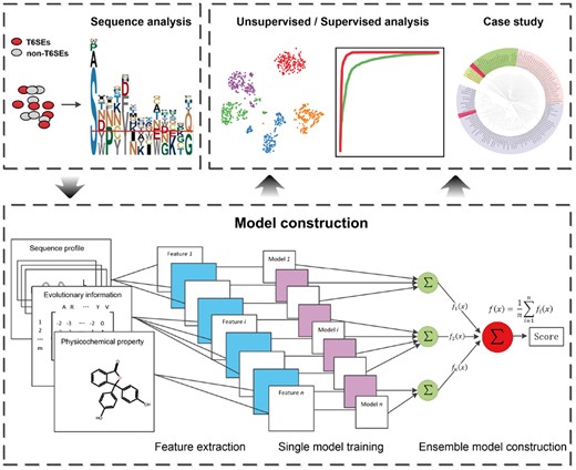
Workflow of our developed Bastion6 approach

2.1 Data collection and preprocessing

To construct the training dataset, we extracted 178 known T6SE sequences from the SecretEPDB database (An et al., 2017) and 1132 non-effectors from the literature (Zou et al., 2013), and then removed highly homologous sequences at the threshold of 90% sequence identity due to limited positive samples. We finally obtained a training dataset containing 138 positive and 1112 negative protein sequences (Supplementary Fig. S1).

To further evaluate the performance of our proposed ensemble method, as compared with single feature based models and existing motif-based T6SE searching methods, we generated an independent dataset by extracting T6SEs from recently published works in the literature (Supplementary Table S1) and non-T6SEs from Vibrio parahaemolyticus. After highly homologous samples (with more than 90% similarity) were removed from our training dataset, we obtained the final independent dataset with 20 positive and 200 negative samples. Aside, two very recently experimentally validated T6SEs (Lin et al., 2017; Si et al., 2017) were used as case studies to test the identifying capability of the proposed method.

2.2 Feature extraction

A protein’s amino acid sequence contains important intrinsic information that dictates its properties. These include composition, permutation and combination modes of amino acids, orders of amino acids, similarities, homologies with other proteins, evolutionary information and physicochemical properties. While each type of feature may contribute to the characteristics of T6SEs, none of the features is predominant among all T6SEs, or indeed constitutes a sufficient and necessary determinant for a protein to be an effector. Thus, extracting features from a wide range of properties would better characterize T6SEs. In this work, we categorized this information into three groups: sequence profile, evolutionary information and physicochemical property.

2.2.1 Group 1: sequence-based features

Protein function is determined by the three-dimensional structure of the protein itself, which in turn depends on the primary structure, i.e. amino acid sequence (Anfinsen, 1972). Different proteins differ in the percentage compositions of amino acids, the modes of combination of amino acids, and the orders of amino acids. Accordingly, three types of sequence-derived features, including amino acid composition (AAC), dipeptide composition (DPC) and Quasi-Sequence-Order descriptors (QSO), were encoded to represent the above characteristics, respectively.

1. AAC is a widely used type of characterizing the occurrence frequencies of 20 amino acids in a sequence and can thus generate a 20-dimensional feature vector.

2. DPC describes the frequencies of dipeptides, each of which is made up of a pair of amino acids. It thus generates a 400-dimensional feature vector, which partially reflects the sequence order information and fragment information.

3. QSO (Chou, 2000) describes the sequence order effect based on the physicochemical distance between amino acids. The QSO descriptors of the sequence can be calculated as:

   $$\left\{\begin{array}{l}{X}_r=\frac{f_r}{{\sum }_{r=1}^{20}{f}_r+\omega {\sum }_{d=1}^{maxlag}{\tau }_d}, r=1,2,\dots ,20,\\ X_d=\frac{{\omega \tau }_{d-20}}{{\sum }_{r=1}^{20}{f}_r+\omega {\sum }_{d=1}^{maxlag}{\tau }_d}, d=21,22,\dots ,20+maxlag,\\ {\tau }_d=\sum _{i=1}^{N-d}{\left({dist}_{i,i+d}\right)}^2,d=1,2,\dots ,maxlag,\end{array}\right.$$

where $f_r$ represents the normalized occurrence for amino acid r, ${dist}_{i,i+d}$ denotes the distance between the ith amino acid and the (i + d)th amino acid of the sequence, N counts the amino acids of the sequence, $\omega$ denotes the weighting factor and maxlag defines the maximum lag that should be no more than the length of the protein sequence. Accordingly, by applying these formulas into Schneider-Wrede physicochemical distance matrix (Schneider and Wrede, 1994) and another chemical distance matrix (Grantham, 1974), two feature vectors were obtained, each of which combines $X_r$ and $X_d$ in 20 + maxlag dimensions, with default values $\omega$ = 0.1 and maxlag = 30.

2.2.2 Group 2: evolutionary information-based features

An increasing number of studies have shown that including evolutionary information is more informative than just sequence information alone (An et al., 2018; Wang et al., 2017a; Zou et al., 2013). Accordingly, such information can serve as a basis for additional feature encodings (Wang et al., 2017b):

1. The Blocks substitution matrix (BLOSUM) is a substitution matrix used to score local alignments between evolutionarily divergent protein sequences. Due to its usefulness it has been applied in many previous bioinformatics studies (Capra and Singh, 2008; Jones, 1999; Jones and Cozzetto, 2015; Wen et al., 2016). In this work, we encoded a protein sequence by mapping its amino acids onto the BLOSUM62 matrix to retrieve the residue similarity values. Accordingly, we obtained a 175-dimentional feature vector.

2. A position-specific scoring matrix (PSSM) is a L × 20 matrix, where L is the length of its corresponding protein sequence. The (i, j)th element of the matrix denotes the probability of amino acid j to appear at the ith position of the protein sequence (Wang et al., 2017a). By borrowing the idea of a DPC encoding algorithm and applying it to a PSSM, DPC-PSSM is designed to partially express the local sequence-order effect (Liu et al., 2010). As a result, DPC-PSSM is represented by a 400-dimentional feature vector, which utilizes the evolutionary information and, moreover, reflects the sequence-order information. DPC-PSSM can be calculated as:

$\left\{\begin{array}{l}Y={\left(y_{1,\mathrm{\hspace{0.17em}}1},{\dots ,y}_{1,\mathrm{\hspace{0.17em}}20},y_{2,\mathrm{\hspace{0.17em}}1},\dots ,y_{2,\mathrm{\hspace{0.17em}}20},\dots ,y_{20,\mathrm{\hspace{0.17em}}1},\dots ,y_{20,\mathrm{\hspace{0.17em}}20}\right)}^T\\ y_{i,j}=\frac{1}{L-1}\sum _{k=1}^{L-1}{p}_{k,i}\times p_{k+1,j} \left(1\le i,j\le 20\right)\end{array}\right.$

where $p_{k,i}$ denotes the element at kth row and ith column of PSSM, and L denotes the row counts of the PSSM, which is equal to the length of the corresponding protein sequence.

• 3.S-FPSSM is designed to extract evolutionary information delicately based on the matrix transformation of the original PSSM (Zahiri et al., 2013). The ‘filtered’ matrix FPSSM is produced from PSSM in a preprocessing step during which all negative elements of the PSSM are set to zero and all positive elements greater than an expected value δ (with a default value of 7) are set to δ. Consequently, all elements in FPSSM are in the range from 0 to δ. This step can help eliminate the negative elements’ influence on the positive ones when adding two elements during matrix transformation. Based on the FPSSM, the resulting feature vector $\mathrm{S}=({\mathrm{S}}_1^{\left(1\right)},\dots ,{\mathrm{S}}_{20}^{\left(1\right)},\dots ,{\mathrm{S}}_1^{\left(20\right)},\dots ,{\mathrm{S}}_{20}^{\left(20\right)})$ can be defined as follows:

$s_j^{\left(i\right)}=\sum _{k=1}^L{fp}_{k,j}\times {\delta }_{k,i}$

subject to

$\left\{\begin{array}{l}{\delta }_{k,i}=1, r_k=a_i\\ {\delta }_{k,i}=0, r_k\ne a_i\end{array}\right.\mathrm{ }i,j=1,\dots ,20$

where L denotes the total number of rows of the FPSSM, ${fp}_{k,i}$ denotes the element in the kth row and ith column of FPSSM, $r_k$ denotes the kth residue in the sequence, and $a_i$ denotes the ith amino acid of 20 primary amino acids.

• 4.Pse-PSSM was originally proposed by Chou et al. and many empirical studies demonstrated its usefulness in protein sequence analysis (Chou and Shen, 2007). It is a reliable feature encoding method for extracting evolutionary information based on the PSSM transformation, and dimension normalization of the resulting feature vector. Pse-PSSM can be described using the following formulae:

${mean}_i=\frac{{\sum }_{k=1}^{20}{E}_{i,k}}{20},\mathrm{ }i=1,2,\dots ,L$

${STD}_i=\sqrt{\frac{{\sum }_{u=1}^{20}\left(E_{i,u}-{mean}_i\right)}{20}\mathrm{ }},\mathrm{ }i=1,2,\dots ,L$

$T_{i,j}=\frac{E_{i,j}-{mean}_i}{{STD}_i},\mathrm{ }i=1,2,\dots ,L$

$H_j^{\alpha }=\frac{1}{L-\alpha }\sum _{i=1}^{L-\alpha }{(T_{i,j}-T_{i+\alpha ,j})}^2$

$\overline{T_j}=\frac{1}{L}\sum _{i=1}^L{T}_{i,j}$

$T^{\mathrm{\text{'}}}=[\overline{T_1},\dots ,\overline{T_{20}}]$

$H^{\mathrm{\text{'}}}=[H_1^{\alpha },\dots ,H_{20}^{\alpha }]$

$P_{PsePSSM}^{\alpha }=[T^{\mathrm{\text{'}}},H^{\mathrm{\text{'}}}]$

where $E_{i,k}$ denotes the element in the ith row and kth column of the original PSSM, and L denotes the length of the protein sequence. Consequently, Pse-PSSM can be represented as a 40-dimentional feature vector, which reflects the relationship between an amino acid and its following αth amino acid in the sequence. In this work, we used the default value $\alpha =1$⁠.

2.2.3 Group 3: physicochemical features

We included two types of physicochemical properties [i.e. composition, transition and distribution (CTD)], composition among CTD (termed as CTDC) and transition among CTD (termed as CTDT) (Xiao et al., 2015), which were previously designed to describe the global composition of amino acid properties in protein sequence (Dubchak et al., 1995).

1. There are seven types of physicochemical properties in this work. For each property, 20 primary amino acids are categorized into 3 different classes, according to their attributes (Table 1). Thus, CTDC is represented as a 21-dimentional feature vector, obtained from a protein sequence, as follows:

   Table 1.

   Classification of 20 standard amino acid types according to seven specific types of physicochemical properties

   	Class 1	Class 2	Class 3
   Hydrophobicity	Polar R, K, E, D, Q, N	Neutral G, A, S, T, P, H, Y	Hydrophobicity C, L, V, I, M, F, W
   Normalized van der Waals volume	0–2.78 G, A, S, T, P, D, C	2.95–4.0 N, V, E, Q, I, L	4.03–8.08 M, H, K, F, R, Y, W
   Polarity	4.9–6.2 L, I, F, W, C, M, V, Y	8.0–9.2 P, A, T, G, S	10.4–13.0 H, Q, R, K, N, E, D
   Polarizability	0–0.108 G, A, S, D, T	0.128–0.186 C, P, N, V, E, Q, I, L	0.219–0.409 K, M, H, F, R, Y, W
   Charge	Positive K, R	Neutral A, N, C, Q, G, H, I, L, M, F, P, S, T, W, Y, V	Negative D, E
   Secondary Structure	Helix E, A, L, M, Q, K, R, H	Strand V, I, Y, C, W, F, T	Coil G, N, P, S, D
   Solvent Accessibility	Buried A, L, F, C, G, I, V, W	Exposed R, K, Q, E, N, D	Intermediate M, S, P, T, H, Y

$C_A=\frac{n_A}{N},\mathrm{ }A=1,2,3$

where $n_A$ denotes the number of amino acid type (class) A, and N denotes the sequence length.

• 2. CTDT is a representation of the frequency with which a type A residue is followed by a type B residue, or vice versa. Accordingly, CTDT is a 21-dimentional feature vector and can be calculated as follows:

  $$\left\{\begin{array}{l}{T}_{AB}=\frac{n_{AB}+n_{BA}}{N-1}\\ T_{BC}=\frac{n_{BC}+n_{CB}}{N-1}\\ T_{CA}=\frac{n_{CA}+n_{AC}}{N-1}\end{array}\right.$$

where $n_{AB}$ denotes the number of dipeptide AB in the sequence, and N denotes the length of the sequence.

2.3 Integrative model construction

To address the imbalanced classification problem, we constructed N (N = 100 in our setting) SVM classifiers and trained each of them with a different subset of the training dataset (Chen and Jeong, 2009). More specifically, to construct an individual classifier, all the positive samples and an equal number of negative samples randomly selected from the training dataset were combined as training samples. For each SVM classifier, we adopted the Gaussian radial basis kernel and performed a grid search to optimize the two parameters, Cost (C) and $Gamma\mathrm{ }(\gamma )$⁠, in the search space $\left\{2^{-10},\dots ,2^{10}\}\right\}$⁠. Thus, for each feature, an ensemble SVM classifier (termed as single feature-based model) was generated by averaging the prediction scores of all the N SVM classifiers. In this way, the imbalanced classification problem is transformed and replaced by multiple balanced data classification problems.

Different features correspond to different properties of proteins and thus can be viewed as capturing distinct protein characteristics from various perspectives, thereby resulting in different data distributions (Chen and Jeong, 2009). Incorporating such knowledge may help improve the prediction performance, as compared to models that have been trained using a single feature only. For each group of features, the prediction scores of single feature based models are averaged to obtain a one-layer ensemble model. Lastly, prediction scores of these one-layer ensemble models (corresponding to different feature groups) are averaged to form an integrative two-layer ensemble model for the final prediction (Fig. 1).

2.4 Performance evaluation

To measure the performance of the proposed method, we carried out an unsupervised analysis, a supervised analysis (including 5-fold cross-validation and independent tests) and case studies. Five performance measures including SN, SP, ACC, F-value and MCC were used. These are defined as follows:

$$SN=\frac{TP}{TP+FN}$$

$$SP=\frac{TN}{TN+FP}$$

$$ACC=\frac{TP+TN}{TP+FP+TN+FN}$$

$$F-value=2\times \frac{TP}{2TP+FP+FN}$$

$$MCC=\frac{\left(TP\times TN\right)-(FN\times FP)}{\sqrt{(TP+FN)\times (TN+FP)\times (TP+FP)\times (TN+FN)}}$$

where $TP$⁠, $TN$⁠, $FP$ and $FN$ denote the numbers of true positives, true negatives, false positives and false negatives, respectively.

3 Experimental results

3.1 Sequence analysis

One of the current tools for T6SE discovery is a motif-based search called MIX (marker for type six effectors) focused on N-terminal sequence similarities found in a sample of T6SEs from Vibrio parahaemolyticus (Salomon et al., 2014), and together with other analysis has suggested common features may be present more broadly in the N- and C- terminal sequences of T6SEs (Lien and Lai, 2017). To test this hypothesis, a sequence analysis was conducted to characterize the amino acid occurrences on the first 50N-terminal and 50C-terminal positions of T6SEs (Supplementary Fig. S2A). The calculated amino acid frequencies show no indication for a strongly conserved sequence motif at either end of the proteins. Indeed, the only discernible position with a high conservation level (bit count twice as high as the second highest stack) is found at position 1 of the N-terminal sequences. However, a similarly high conservation is also found for non-effector proteins (Supplementary Fig. S2B), which can be distinguished at that position only by the relative abundance of lysine (K) and phenylalanine (F) residues and a depletion in proline (P) and arginine (R) residues. The C-terminal amino acids of both T6SEs and non-effectors show a distinctively even conservation distribution, indicating that none of the positions plays a major role in recognition. A more than twofold increase compared to the average stack height is only observed for the very last position of non-effector proteins, which is enriched in lysine (K) and glutamate (E), but depleted in leucine (L).

3.2 Unsupervised analysis

To intuitively visualize the effect of different feature encodings on the classification performance, we conducted an unsupervised analysis based on a randomly selected balanced dataset (due to the impossibility of visualizing all N balanced datasets) and demonstrated the value of such analysis to ascertain whether the extracted features can be used to effectively discriminate the T6SEs from non-effectors (Hulsman et al., 2014). For each feature encoding, we mapped all the samples (including both positives and negatives) onto the 2D space (Fig. 2), so that the differences in the characterization of these samples would be represented by their mutual distances in space. Although the samples from both classes are not evenly distributed across the 2D map, the embedding didn’t show a clear division into distinct subgroups. To further investigate this, the data was processed using K-means clustering. In this way, the samples in the picture were colored by their clustering labels, and shaped by the true labels. The classified distribution of the data samples in each cluster is shown as the bar chart in Figure 2 (with detailed results listed in Supplementary Table S2).

Fig. 2.

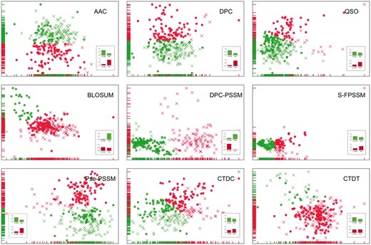
Representation and clustering of data samples of T6SEs and non-T6SEs based on nine different types of feature encodings. For each encoding, the representation of data samples is presented in two dimensions after dimensionality reduction using principal component analysis (PCA). Samples were then clustered into two groups using the K-means algorithm; each cluster (represented by one color) consists of two types of samples (i.e. T6SEs and non-T6SEs) with two different shapes, in which circle and multiplication signs represent T6SEs and non-T6SEs, respectively. The classified distribution of T6SEs (right-hand bar) vs. non-T6SEs (left-hand bar) in each cluster is shown as the inset bar chart

DPC-PSSM outperformed all other feature encoding methods: using DPC-PSSM, non-T6SEs dominated in Cluster 1 (accounting for 99.1%) while T6SEs dominated in Cluster 2 (accounting for 84.6%). The apparently higher division and low mixture rate of two classes of samples in each cluster strongly demonstrated the ability of this encoding scheme to recognize the T6SEs from non-effectors. Following DPC-PSSM, DPC, AAC and Pse-PSSM achieved a good, comparable performance, with a moderate mixture rate within each cluster. The good performances of these four encoding methods illustrate that evolutionary information-based and sequence-based features contribute the most to T6SE classification.

Note that although T6SEs dominated in Cluster 2 (96.9%) for BLOSUM, there was a considerable number of T6SEs and non-T6SEs aggregated together in Cluster 1 (43.9% of T6SEs and 56.1% of non-T6SEs). Moreover, there was an imbalance between Cluster1 (containing 244 samples) and Cluster 2 (containing 32 samples) which could potentially impact the classification outcome.

3.3 Supervised analysis

We further evaluated the effect of each feature encoding in a supervised setting, enabling us to quantitatively assess them by using a set of standard measures on 5-cross validation and independent tests. All 5-fold cross validation tests in this work were conducted based on N (N = 100 in our setting) balanced training datasets, and the performance was averaged over these N balanced datasets.

3.3.1 Performance evaluation using 5-fold cross-validation tests

For each feature encoding method, an SVM classifier was trained with optimally-tuned parameters and validated based on the training dataset by performing randomized 5-fold cross-validation tests. The averaged results are shown in Table 2 and Figure 3A.

Table 2.

The performance of SVM classifiers using different sequence encoding methods based on 5-fold cross-validation tests

	Encoding	SN	SP	ACC	F-value	MCC
Group 1	AAC	0.871±0.022	0.875±0.028	0.873±0.020	0.872±0.020	0.748±0.041
	DPC	0.837±0.020	0.852±0.027	0.843±0.020	0.841±0.020	0.689±0.039
	QSO	0.843±0.020	0.863±0.027	0.851±0.018	0.849±0.018	0.706±0.036
Group 2	BLOSUM	0.810±0.034	0.796±0.031	0.802±0.024	0.803±0.025	0.608±0.048
	DPC-PSSM	0.950±0.020	0.929±0.019	0.938±0.013	0.940±0.013	0.878±0.025
	S-FPSSM	0.915±0.014	0.918±0.020	0.914±0.012	0.915±0.012	0.831±0.024
	Pse-PSSM	0.925±0.015	0.944±0.019	0.932±0.012	0.933±0.012	0.868±0.023
Group 3	CTDC	0.857±0.025	0.847±0.033	0.850±0.021	0.851±0.020	0.705±0.042
	CTDT	0.774±0.031	0.764±0.030	0.771±0.024	0.767±0.026	0.544±0.049

Note: The values were expressed as mean ± standard deviation. For each metric, the best performance value across different encoding methods is highlighted in bold for clarification.

Fig. 3.

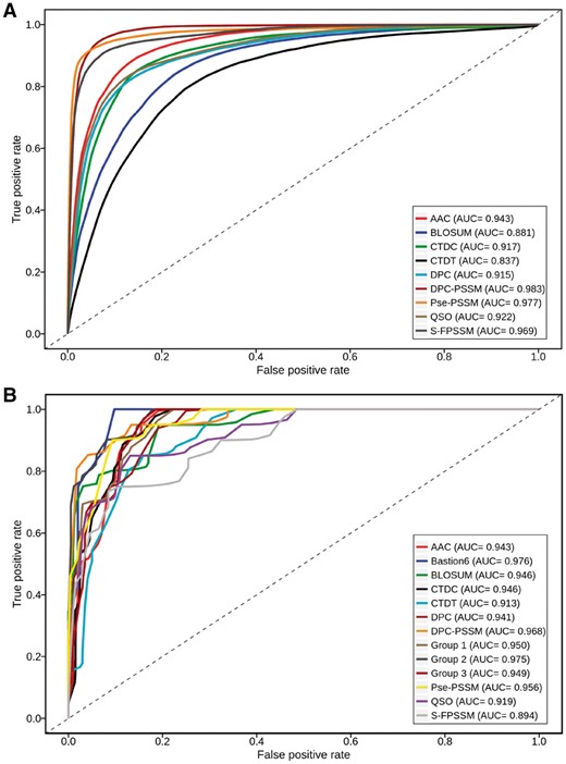
(A) ROC curves of different feature encoding methods for T6SS effector prediction based on 5-fold cross-validation tests; (B) ROC curves of single feature-based models, one-layer models and the final model used by Bastion6 on the independent test. The results were distinguished by color curves. AUC values for each model are also presented

As can be seen, PSSM-based features achieved the overall best performance in terms of ACC (>0.91), F-value (>0.91), MCC (>0.83) and AUC (>0.96) (Table 2 and Fig. 3A). This suggested that PSSM-based features were the most informative for T6SE classification, and its related features were considered as essential for building accurate models. These observations agree well with previous bioinformatics studies (An et al., 2018; Wang et al., 2017a; Zou et al., 2013). DPC-PSSM was shown to be the most powerful feature encoding method, which consistently achieved the highest values of SN (0.950), ACC (0.938), F-value (0.940), MCC (0.878) and AUC (0.983). These results are in accordance with those in our unsupervised analysis. Similarly, following the PSSM-based feature encoding, AAC achieved the second-best performance reflected by the ACC (0.873), F-value (0.872), MCC (0.748) and AUC (0.943). The poorer performance of BLOSUM indicates that the substitution matrix was less informative when compared with the PSSM, although the former is more accessible and can be directly calculated. The same holds for CTDT, which yielded only a moderate performance, despite it providing a novel perspective on the feature extraction of protein sequences. These results suggest that BLOSUM and CTDT can be used as complementary encoding schemes in conjunction with the essential PSSM features.

Our supervised analysis also revealed differences with respect to the unsupervised analysis. In particular, we found that CTDC and QSO achieved an equivalent performance as the second-best feature encoding methods (with a performance that was slightly better than that of DPC). This suggests that the performance of individual encoding schemes may depend on the machine learning method being applied.

Generally, while there is a preference for high SN and SP values, a trade-off between SN and SP is necessary for a predictor to achieve a comprehensive and stable performance. Otherwise, it could generate predictions that are biased by a preference for a certain class of samples. In this work, the gaps between SN and SP were minor across all the encoding methods, which formed a solid basis for our model to achieve a stable performance over all metrics, including ACC, F-value, MCC and AUC.

3.3.2 Performance evaluation using various sequence similarity rates

Considering that the features used for training the models were derived from protein sequences, the training datasets curated with different sequence similarity cut-offs could result in different model performances. To examine the effect of the sequence similarity cut-off on the overall performance of the models, six sequence identity thresholds (i.e. 70, 75, 80, 85, 90 and 95%) were applied when constructing training datasets. Using these generated datasets and the original dataset (without homologous sequence reduction), the performance of each model was evaluated using the same fivefold cross-validation. As can be seen from Figure 4A, in all cases, the models trained with the original dataset outperformed those trained with other datasets (i.e. after removal of homologous sequences) in terms of the MCC value. This suggests that high sequence homology in the original dataset can indeed lead to overestimated performances of the corresponding models, thereby highlighting the importance and necessity of performing sequence homology reduction prior to model training. However, models trained with datasets resulting from different sequence similarity cut-offs show a similar performance, indicating the robustness of the proposed models.

Fig. 4.

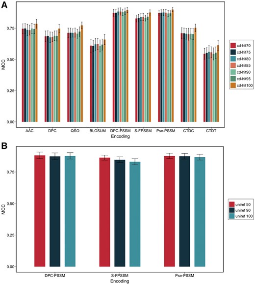
(A) Performance of various feature encoding methods using different sequence similarity cut-offs based on 5-fold cross-validation tests; (B) Performance of various PSSM-based feature encoding methods against different uniref databases based on 5-fold cross-validation test

3.3.3 The effect of searched databases for PSSM-based features

To characterize the potential effect of the size of searched databases on the performance of PSSM-based models, we further generated PSSM profiles by searching against three uniref databases with different sizes (i.e. uniref50, uniref90 and uniref100) with parameters of j = 3 and h = 0.001. Based on these PSSM profiles, PSSM-based models were trained and performance evaluated using the same fivefold cross-validation procedure. The results indicate that there was no significant difference in the performance between these PSSM-based models (Fig. 4B), suggesting that the size of searched databases did not have a significant impact on the performance of the PSSM-based models on the curated T6SE dataset.

3.3.4 The effect of various selected features on the model performance

GainRatio (Frank et al., 2004) was applied to conduct a set of feature selection experiments using the same fivefold cross-validation. We found that for different types of features, models trained using the entire features generally resulted in a better predictive performance compared to models trained using selected features (such as the top 50, 100, 150, 200, 250, 300 and 350 features) (Supplementary Fig. S3). The only exception was the BLOSUM-based model, which achieved a similar performance when compared to the corresponding model trained using selected features. A possible explanation is that the original size of each generated feature set was so small (i.e. less than 400 dimensions) that all features in the feature set without further selection could be interpreted well by machine learning methods, contributing to the models’ overall performance.

3.3.5 Comparison with homology-based baseline predictor

To compare with the proposed models, we applied a homology-based approach to develop a baseline predictor. For each query sequence in the test set, the blastp program—implemented in the Blast+ software (Camacho et al., 2009)—was used to search against the training dataset. Based on the blastp search results, the query sequence was assigned the same label as that of the top ranked protein sequence with the lowest E-value in the training dataset. We thus assessed the performance of this homology-based baseline predictor using the same fivefold cross-validation. The results showed that the baseline predictor achieved a lower performance with an F-value of 0.787, an ACC of 0.741 and an MCC of 0.517, than our proposed models. An explanation is that the homology-based baseline predictor could not recognize valuable patterns beyond the sequence identity, thus resulting in an unsatisfactory performance compared with our machine learning-based models.

3.3.6 Performance validation on the independent test

Using the independent test, the proposed two-layer ensemble model was further assessed, and benchmarked against the single feature-based, one-layer ensemble models. All experiments were conducted 10 times. Each time, a balanced independent dataset was formed by the positive samples and 20 randomly chosen negative samples. As shown in Figure 3B and Supplementary Table S3, most of the ensemble models display a better and more stable performance in terms of ACC, F-value, MCC and AUC, when compared to their single feature-based models, while Bastion6 achieved the best performance among them with respect to ACC (0.943), F-value (0.946), MCC (0.892) and AUC (0.976).

To measure the ability of positive sample identification, we further looked into the numbers of true positives predicted by various models in the independent test. Bastion6 outperformed the single feature-based models and one-layer ensemble models (Supplementary Table S4), without misclassifying any T6SE. In contrast, single feature-based models misclassified a larger number of T6SEs. As expected, ensemble models were able to correct the misclassifications of single feature-based models, and consequently achieved more stable performances.

Two previous motif search-based methods were assessed as a benchmark for the independent test, since motif strategies referred to as MIX and SAVC (Secretome analysis of Vibrio cholera) were recently used to discover T6SEs (Altindis et al., 2015; Salomon et al., 2014). Regarding the capability of recognizing T6SEs, Bastion6 successfully retrieved 20 positive samples, while MIX and SAVC retrieved 0 and 2 positive samples, respectively, from 20 T6SEs of the independent dataset (Supplementary Table S5). This result suggested that motif-based searching methods do not function well across bacterial species, and demonstrated the usefulness and necessity of our universal and highly accurate T6SE prediction method.

3.4 Case study

To examine the scalability and robustness of the proposed method, we carried out a case study using two very recent experimentally validated T6SEs: neither of these effectors was present in the training dataset, and both differ significantly from all other proteins in the training dataset (Supplementary Figs S4 and S5). Detailed prediction results are listed in Supplementary Table S6.

Our first case study protein was TseM (Si et al., 2017), a T6SS-4–dependent Mn²⁺-binding effector experimentally characterized from Burkholderia thailandensis. The proposed model correctly identified TseM as a T6SE, with a probability score of 0.544. As a comparison, models trained using sequence-based features generated lower probability scores (<0.5) due to the low sequence similarity between TseM and the protein sequences in the training dataset (Supplementary Figs S4 and S5). Models trained using PSSM (except S-FPSSM) and physicochemical properties could correctly recognize TseM as a T6SE with higher prediction scores. More specifically, the CTDT model correctly predicted this protein with the highest score of 0.763, despite its poorer performance in benchmarking experiments.

The second case study was the T6SE TseF recently identified in Pseudomonas aeruginosa (Lin et al., 2017). TseF is secreted by the H3-T6SS, and then incorporated into outer membrane vesicles to facilitate the uptake of iron (Lin et al., 2017). The proposed model successfully predicted TseF as a T6SE with a score of 0.681. Surprisingly, DPC-PSSM and Pse-PSSM models, which performed best in benchmarking experiments, failed to predict this T6SE. This highlights the necessity of exploiting the different but complementary feature encoding schemes that can capture useful ‘signals’ from different perspectives.

These results confirm the usefulness and reliability of our proposed method, and the value of integrating various models into ensemble learning models. By taking all these single models into account, the developed two-layer model achieved balanced predictive power, thus providing a reliable tool for identifying novel potential T6SEs.

3.5 Genome-scale prediction across various species

Currently, there are only a limited number of experimentally validated T6SEs. This has restricted our understanding of the functional roles in their interactions with their eukaryotic hosts or prokaryotic competitors. To facilitate the functional characterization, we performed a genome-wide prediction of T6SEs in 12 different bacterial species, including those that have been previously shown to possess T6SEs. As a result, a total of 94 putative T6SEs (with probability scores larger than 0.9) were extracted from 54 212 protein sequences. A statistical summary of the genome-wide prediction results is listed in Supplementary Table S7. A full list of the predicted T6SEs can be found at the Bastion6 server.

4 Discussion

Identification of T6SEs is a key to understanding the role of T6SS in bacteria’s anti-bacterial competition, inter-bacterial interaction and virulence to their eukaryotic hosts (Ho et al., 2014). Bacterial genome sequencing is advancing at an unprecedented pace and, consequently, rapid and accurate identification of T6SEs from genome sequence data is both achievable and highly desirable. Previous studies have reported motifs in N- or C-terminal sequences in some bacterial (Lien and Lai, 2017) suggested to define T6SEs. However, these motifs prove to be specific to a subset of T6SEs in only certain bacterial species. The latter was shown through sequence analysis and further validated in the benchmark tests in this work. To provide highly accurate prediction of T6SEs in and across diverse bacterial species, we extracted nine widely used features based on amino acid sequence information, evolutionary information and physicochemical properties. These features have been systematically and comprehensively assessed through unsupervised and supervised learning. The features demonstrated their effectiveness in different scenarios. PSSM-based features achieved the overall best performance in most cases. They could accurately predict novel T6SEs especially in cases where they significantly differ from known effectors. However, we also noticed that in some cases, PSSM-based features did not perform well while other features performed better on independent tests and case studies. There might be several reasons for this. First, compared to the vast number of uncharacterized effectors the dataset of known T6SEs was very limited when it comes to extracting sufficient knowledge and useful patterns. Accordingly, it was hard to quantitatively assess how a feature performs, relative to other features. Second, different features may be suitable for predicting different T6SEs. A feature-based model may be good at recognizing a subset of T6SEs while it fails to identify another subset of T6SEs. Therefore, taking advantage of all single feature-based models and integrating them into an ensemble model helps to improve the prediction of T6SEs.

The relatively small number of T6SE samples in the benchmark dataset will likely result in some bias in the prediction performance. However, the discovery of new T6SEs: bioinformatically, genetically and through other experimental approaches, will expand the benchmark dataset and, accordingly, improve the model by lessening any potential bias. Additionally, other features that have proved useful in other bioinformatics studies (such as structure-based features and GO-based features) may help identify new patterns and improve the model once more T6SE data becomes available.

In this study, we have developed Bastion6, a two-layer ensemble machine learning method integrating a number of individual SVM-based models. Extensive benchmarking experiments validated the effectiveness and robustness of our proposed model. We further applied Bastion6 to perform genome-wide predictions and obtained a list of high-confidence, putative T6SEs in 54 212 proteins across 12 bacterial species. With these promising results, we believe our predicted T6SEs can serve as a preliminary screen for follow-up experiments. In addition, we implemented a publicly accessible web server, to meet users’ specific demands. We believe that our proposed method can be a vastly useful tool for T6SE prediction, and will expedite the discovery of novel T6SEs.

Acknowledgements

We thank Dr. Jonathan Wilksch, Dr. Romé Voulhoux and Dr. Badreddine Douzi for critical comments on the manuscript.

Funding

This work was supported by grants from the National Health and Medical Research Council of Australia (NHMRC) (1092262), the Australian Research Council (ARC), the National Institute of Allergy and Infectious Diseases of the National Institutes of Health (R01 AI111965) and the Natural Science Foundation of Guangxi Under No. 2016GXNSFCA380005. AL and TML were supported by informatics startup packages through the UAB School of Medicine. T.L. is an ARC Australian Laureate Fellow (FL130100038).

Conflict of Interest: none declared.