Deep learning improves antimicrobial peptide recognition

Abstract

Motivation

Bacterial resistance to antibiotics is a growing concern. Antimicrobial peptides (AMPs), natural components of innate immunity, are popular targets for developing new drugs. Machine learning methods are now commonly adopted by wet-laboratory researchers to screen for promising candidates.

Results

In this work, we utilize deep learning to recognize antimicrobial activity. We propose a neural network model with convolutional and recurrent layers that leverage primary sequence composition. Results show that the proposed model outperforms state-of-the-art classification models on a comprehensive dataset. By utilizing the embedding weights, we also present a reduced-alphabet representation and show that reasonable AMP recognition can be maintained using nine amino acid types.

Availability and implementation

Models and datasets are made freely available through the Antimicrobial Peptide Scanner vr.2 web server at www.ampscanner.com.

Supplementary information

Supplementary data are available at Bioinformatics online.

1 Introduction

Antimicrobial resistance remains a serious problem for humans and livestock around the world, as more drugs lose sensitivity to the pathogens they were designed to eliminate (Price et al., 2012; U.S. Department of Health and Human Services, 2013; World Health Organization, 2014). Over the past few decades, natural antimicrobial peptides (AMPs) have been an active area of research and have shown a lowered likelihood for bacteria to form resistance compared to many conventional drugs (Boman, 2003; Zelezetsky et al., 2006). AMPs are short innate immunity peptides that fall into a number of diverse sequence families (e.g. cathelicidins, defensins, cecropins, etc.) and kill their targets through various mechanisms, such as cell membrane damage, DNA interference or signaling for adaptive immune responses, as reviewed by Wimley and Hristova (2011). While we focus in this work exclusively on peptides that kill Gram-positive and/or Gram-negative bacteria, we note some AMPs have also been shown effective against a variety of fungal and viral pathogens (Wang, 2010).

To aid wet-laboratory researchers in novel AMP discovery, a variety of computational approaches are proposed for AMP recognition. Many incorporate machine learning algorithms or statistical analysis techniques, such as artificial neural networks (ANN) (Lata et al., 2010; Thomas et al., 2009; Torrent et al., 2011), discriminant analysis (DA) (Thomas et al., 2009), fuzzy k-nearest neighbor (Xiao et al., 2013), hidden Markov models (Fjell et al., 2009), logistic regression (Veltri et al., 2017; Randou et al., 2013), random forests (RF) (Thomas et al., 2009; Veltri, 2015) and support vector machines (SVM) (Lata et al., 2010; Lee et al., 2016; Meher et al., 2017; Thomas et al., 2009; Torrent et al., 2011).

Popular features/predictors for peptide sequences are based on sequence composition. Basic amino acid counts over the N- and C-termini or the full peptide are used by the AntiBP (Antibacterial Peptide) methods (Lata et al., 2007, 2010). The pseudo-amino acid composition (PseAAC) method (Chou, 2001) also incorporates information about sequence order (Meher et al., 2017; Xiao et al., 2013). In the evolutionary feature construction (EFC) method (Kamath et al., 2014), features encode nonlocal correlations between position-specific sequence motifs (Veltri et al., 2017, 2014).

Physicochemical properties, such as charge, hydrophobicity, isoelectric point, aggregation propensity and more, are also used to encode sequences as numerical vectors; typically, features are average values of considered physicochemical properties calculated over the full-length or terminal ends of a peptide sequence (Fernandes et al., 2012; Randou et al., 2013; Thomas et al., 2009; Torrent et al., 2011). While a few methods attempt to numerically predict the ‘strength’ of antimicrobial activity (i.e. inhibition concentration) (Cherkasov and Jankovic, 2004), most methods use a binary prediction/recognition setting to assign an ‘AMP’ or ‘non-AMP’ label to a given query peptide sequence.

Many AMP recognition methods are provided to the research community via web servers. Recent ones include iAMPpred (Meher et al., 2017), iAMP-2 L (Xiao et al., 2013), AntiBP2 (Lata et al., 2010), CAMP (Thomas et al., 2009) and AMPer (Fjell et al., 2007). Reported recognition accuracy (ACC) has steadily improved over the past decade, but there is room for improvement. Comparative surveys report that state-of-the-art servers, including CAMP and AntiBP2, miss many true positives (Bishop et al., 2015; Veltri, 2015). Others, such as the Antimicrobial Peptide Database (APD) (Wang et al., 2016) and AMP predictor, only accept individual query sequences that limit applications for high-throughput recognition experiments by wet-laboratory researchers.

In this paper, we improve upon the state of the art in AMP recognition and make several contributions. First, we offer a new training and testing dataset that reflects the latest available antibacterial peptide data from the recently updated APD vr.3 release. Second, we introduce a new deep neural network (DNN) classifier that achieves better AMP recognition compared to the existing methods. Third, by using a DNN with convolutional (Conv) and recurrent layers, we remove the burden of a priori feature construction and consequently reduce our reliance on domain experts. Fourth, we make the proposed DNN model and all datasets freely available to the research community via the AMP Scanner server at: http://www.ampscanner.com. The server is specifically designed to support high-throughput screening experiments, where wet-laboratory researchers want to conduct systematic virtual screenings of peptide libraries to identify promising peptides for further characterization and modification. Finally, to directly support the design of such libraries, we ‘open’ the box of the proposed DNN model and learn from it a smaller alphabet via which to represent peptide sequences. We demonstrate that the smaller alphabet allows retaining good AMP recognition ACC. Moreover, by reducing the number of amino acids from 20 to 8 pseudo-amino acids (plus a padding character), we shrink the size of the sequence space wet-laboratory researchers have to consider when designing peptide libraries.

The superiority of DNN models has been demonstrated on many problems in bioinformatics. While, to the best of our knowledge, this paper is the first to propose DNN models for AMP classification, other recent DNN models improve protein secondary structure prediction (Spencer et al., 2015), protein fold recognition (Jo et al., 2015), drug discovery and more (LeCun et al., 2015). The interested reader is directed to the survey by LeCun et al. (2015) for a review of deep learning and its performance on diverse problems spanning from genomics to drug discovery.

The DNN model proposed in this paper captures position-invariant patterns along an amino acid sequence through the use of Conv (LeCun et al., 2015) and ‘long short term memory’ (LSTM) layers (Hochreiter and Schmidhuber, 1997) based on a popular architecture in speech recognition tasks (Bahdanau et al., 2014; Vinyals et al., 2015). The proposed DNN uses separate Conv and LSTM layers and is different from the ‘Convolutional LSTM’ architecture outlined recently by Xingjian et al. (2015) for precipitation nowcasting. Our choice of LSTM layers is due to the fact that, as a type of recurrent neural network, LSTMs have the ability to ‘recognize’ and ‘forget’ gap-separated patterns (Schmidhuber, 2015), and they have recently been shown successful in bioinformatics contexts like identifying protein subcellular localization (Nielsen et al., 2016). We note our use of the term ‘deep’ in this work is intended to reflect the structure of our model rather than the number of layers employed.

The rest of this paper is organized as follows. The DNN model and the construction of the reduced alphabet are detailed in Section 2. The model is evaluated in a comparative setting in Section 3, which also evaluates the impact of the reduced alphabet gleaned from the model on recognition ACC. The paper concludes in Section 4.

2 Materials and methods

2.1 Datasets

We build our dataset over experimentally validated AMPs available in the APD vr.3 database (at http://aps.unmc.edu/AP). These AMPs are active against Gram-positive and/or Gram-negative bacteria. We curate this dataset as follows. After filtering out sequences shorter than 10 amino acids in length and those sharing $\ge 90\%$ sequence identity with the CD-HIT program (Huang et al., 2010), we are left with 1778 AMPs. We assign 712 AMPs for training, 354 for tuning/evaluation and 712 for testing, respectively.

As there is currently no large public repository of peptides experimentally shown to lack antimicrobial activity, we build a negative dataset of non-AMP sequences using an approach similar to previous work (Torrent et al., 2011; Xiao et al., 2013). Specifically, we download peptide sequences from UniProt (Magrane and the UniProt consortium, 2011) (http://www.uniprot.org) by setting the ‘subcellular location’ filter to cytoplasm and remove any entry that matches the following keywords: antimicrobial, antibiotic, antiviral, antifungal, effector or excreted. We also remove sequences <10 amino acid in length, those sharing $\ge 40\%$ sequence identity (again, using CD-HIT), or any found to match known AMPs by running a BLAT (Kent, 2002) vr.35 protein-versus-protein search using default settings. We then randomly select 1778 peptide fragments from the remaining sequences, ensuring that the length distribution of the selected non-AMPs approximates that of the AMP dataset constructed as described earlier. The 1778 non-AMPs selected in this manner are assigned to training (712 of them), tuning (354 of them) and testing (712 of them) partitions as done with the AMP dataset.

The Supplementary Information includes the AMP and non-AMP sequence length distributions as well as additional analyses to evaluate the impact of the size and composition of the dataset on model performance. Sequences are available for download in multi-FASTA format from the AMP Scanner web server that accompanies this paper.

2.2 Architecture of proposed DNN

To identify position-invariant AMP sequence patterns, we build a DNN with the Keras framework (http://www.keras.io) using a sequential model and a TensorFlow (Abadi et al., 2016) deep learning library back-end. We consider deep learning due to its ability to identify multiple, ambiguous patterns possibly hiding within the diverse families of AMP peptides represented in our comprehensive dataset. Specifically, the DNN employs Conv and maximal (max) pooling layers to generate filters that generalize sequence patterns and uses an LSTM layer to characterize a possibly highly complex order in which these patterns may occur across various AMPs. An overview of the approach for sequence embedding and DNN architecture is shown in Figure 1.

Fig. 1.

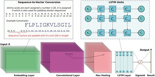
The proposed DNN uses Conv and LSTM layers. Peptide sequences are encoded into uniform numerical vectors of length 200. These vectors (X) are fed to an embedding layer of length 128, followed by a convolutional layer comprised of 64 filters. Each of these filters undergoes a 1D convolution and is downsampled via a maximal pooling layer of size 5. Next, an LSTM layer with 100 units allows the DNN to remember or ignore old information passed along the horizontal dotted arrows extending from each X_i input. The final output from the DNN is passed through a sigmoid function so that predictions (Y) are scaled between 0 and 1

Figure 1 shows that peptide sequences are first converted into zero-padded numerical vectors of length 200 that fit our dataset’s longest AMP (183 amino acids) and non-AMP (175 amino acids). Specifically, each of the 20 basic amino acids are assigned a number 1–20 and unknown ‘X’ characters (not present in any sequence in our dataset) are assigned 0. Since the DNN quickly learns to ignore the leading padding characters, it can handle variable-length sequences. As detailed in Figure 1, such encoded sequences are then fed into an embedding layer (embedding_vector_length: 128 in the Keras framework syntax) and then to a 1D Conv layer (nb_filter: 64, filter_length: 16, init: normal, strides: 1, border_mode: same, activation: relu). The purpose of the embedding layer is to convert the indices of discrete symbols (e.g. amino acids) into a representation of a fixed size vector. For instance, the layer can convert indices (⁠$1,2,\dots ,20$⁠) corresponding to the 20 naturally occurring amino acids into a three-number vector representation. The benefit of the embedding is that it can create a more compact representation of input symbols and can yield semantically similar symbols close to each other in the vector space. The embedding layer can be trained with other layers of a DNN, and its weights can be updated during training.

The 64 filters that are activated when a matching sequence pattern/motif is detected are convolved in a single (forward) direction. A max pooling layer (pool_length: 5) then downsamples these filter values by sliding nonoverlapping windows of length 5 and selecting the largest value. This helps to reduce overfitting and provides slight invariance to residue position. Next, an LSTM layer with 100 units is applied (unroll: True, stateful: False, dropout: 0.1 and rest default settings) which identifies patterns along a sequence that can be separated by large gaps. The LSTM dropout parameter (Srivastava et al., 2014), which helps with overfitting by randomly ignoring 10% of inputs, is used, as it slightly improves the DNN’s predictive performance. Each LSTM unit is comprised of the following gates, where W and U are parameter matrices and b is a bias vector as outlined in Hochreiter and Schmidhuber (1997).

$$\begin{array}{ll}{i}_t=\sigma (W_i{x}_t+U_i{h}_{t-1}+b_i)\hfill & \text{input gate}\hfill \\ {\tilde{C}}_t=\text{tanh}(W_c{x}_t+U_c{h}_{t-1}+b_c)\hfill & \text{candidate cell states}\hfill \\ f_t=\sigma (W_f{x}_t+U_f{h}_{t-1}+b_f)\hfill & \text{forget gate}\hfill \\ C_t=i_t^{\tilde{C}}_t+f_t^C_{t-1}\hfill & \text{cell activation gate}\hfill \\ o_t=\sigma (W_o{x}_t+U_o{h}_{t-1}+V_o{C}_t+b_o)\hfill & \text{output gate}\hfill \\ h_t=o_t^\text{tanh}(C_t)\hfill & \text{hidden gate}\hfill \end{array}$$

Above, $^$ refers to an entry-wise (Schur) product (Davis, 1962). The cell activation gate C is able to consider previous states (⁠$\tilde{C}$⁠), and information is forwarded by f to alter the hidden states h and final output vector o. We note that LSTMs can be implemented so that f passes information in reverse or bidirectionally, but we did not find this to significantly impact recognition performance. In addition, we note that, while the best model we found uses LSTM, similar performance (within 1–2% ACC) was found when replacing LSTM with Gated Recurrent Units (Chung et al., 2014) (another type of recurrent layer). Additional information for the interested reader on the architecture of LSTM and other recurrent layers is available in Hochreiter and Schmidhuber (1997), Gers et al. (2000) and Graves et al. (2013).

Finally, as Figure 1 shows, the output from the LSTM layer is passed through a final dense layer that uses a sigmoid function to force predictions in the range [0, 1]. We compile our Keras model using 10 epochs with the ‘adam’ optimizer (loss: binary_crossentropy, metrics: accuracy). In a 10-fold cross validation (CV) setting, we find that removing the Conv and max pooling layers reduces the ACC by 4% and increases the runtime by approximately 39%.

2.3 Model tuning and construction

As common practice dictates, we build two separate models, first a ‘training’ model used for evaluating the testing partition and second a ‘production’ model for the web server, which is trained on all available data. Model parameters are first tuned through a randomized search using the Hyperas wrapper package (https://github.com/maxpumperla/hyperas) for Keras. The tuning step only uses the training and tuning partitions. After parameters are selected, the training model is built by merging the training and tuning partitions and evaluating performance on the testing dataset. All data partitions are combined to generate the production model and for the 10-fold CV setting with model parameters unchanged. A prediction probability threshold of >0.5 is used to denote an ‘AMP,’ with $\le 0.5$ denoting a ‘non-AMP.”

2.4 Model evaluation

We evaluate classification performance in terms of sensitivity (SENS), specificity (SPEC), ACC and Matthews Correlation Coefficient (MCC), which are defined using the number of true positive (TP), true negative (TN), false-positive (FP) and false-negative (FN) predictions. Specifically, SENS = $TP/(TP+FN)\times 100\%$⁠, SPEC = $TN/(TN+FP)\times 100\%$⁠, ACC = $(TP+TN)/(TP+FP\hspace{0.17em}+TN+FN)\times 100\%$⁠, and MCC = $((TP\times TN)-(FN\times FP))/\sqrt{(TP+FN)\times (TN+FP)\times (TP+FP)\times (TN+FN)}$⁠.

We also make use of the receiver–operating characteristic (ROC) curve (Hanley and McNeil, 1982). The ROC curve shows the performance of a classification model as one varies a discrimination threshold. Specifically, predictions are ranked in descending order, and a threshold value, used to delineate the number of true and false predictions, is adjusted so as to capture the TP rate as a function of the FP rate (Hanley and McNeil, 1982). In addition to drawing the ROC curve, we report the area under the ROC curve (auROC) to evaluate performance in a quantitative, comparative setting. auROC ranges from 0.5 (corresponding to a random guess) to 1 (corresponding to the case when all predictions are correct). We calculate auROC using the pROC vr.1.8 package (Robin et al., 2011) in R (R Core Team, 2015) vr.3.4.1.

2.5 Embedding visualization

To generate the amino acid embedding vector visualization, Conv layer embedding weights are first extracted from the trained Keras model using all the data. Then, t-distributed stochastic neighbor embedding (t-SNE) (Van der Maaten and Hinton, 2008) is applied (n_components: 2, init: pca, perplexity: 30, n_iter_without_progress: 300, method: exact) through the scikit-learn (Pedregosa et al., 2011) vr.0.18.1 package to reduce the original 128D vectors down to two dimensions. Plotting is done using matplotlib (Hunter, 2007) vr.2.0.2.

2.6 Reduced alphabet construction and testing

Clusters are assigned to (amino acid) letters in the embedding using scikit-learn’s k-means algorithm (Lloyd, 1982) (n_clusters: 8) using only the 20 classic amino acids. The setting of k = 8 is selected after plotting the sum of squared distances between samples and cluster centroids for k ranging [1, 19] and looking for a bend based on the elbow method (Thorndike, 1953) (detailed analysis is shown in the Supplementary Information). The nonbiological ‘X’ padding character is manually assigned to its own cluster to bring the total number of clusters to 9.

After a unique letter is randomly chosen to represent each cluster (maintaining the padding cluster as’ X’), a new ‘DNN-reduced’ alphabet is obtained. The DNN model is then trained using the same hyperparameters as above but representing peptide sequences using the DNN-reduced alphabet. This process is repeated 100 times (using different seeds), and ACC and MCC results on the testing dataset (also converted to the new, reduced alphabet) are reported as averages, along with standard deviations (SD) to check for consistency.

To assess whether the DNN-reduced alphabet’s particular cluster membership outperforms random cluster membership, 100 additional ‘randomized’ alphabets are also constructed. For each, ‘X’ is maintained as its own cluster, but the 20 real amino acids are randomly assigned to 8 clusters of the same relative sizes as for the DNN-reduced alphabet. The experiment described above is then repeated, training the DNN model (using the same hyperparameters) on peptide sequences represented using a particular randomized alphabet. Differences in recognition performance between the DNN-reduced and randomized models are evaluated as follows. A two-sample, one-tailed t-test with 95% confidence interval using R is applied to see whether the ACC or MCC means of the 100 DNN-reduced alphabet model classifications are statistically higher than the ACC or MCC means, respectively, of the 100 random alphabet model classifications.

To ensure that findings are applicable beyond DNNs, we repeat the DNN-reduced versus randomized alphabet experiment described above using gkmSVM vr.2.0 (Ghandi et al., 2014). The gkmSVM uses a gapped k-mer SVM algorithm based on sequence composition. Unlike the proposed DNN, the gkmSVM is not stochastic, so only one result per alphabet for a given dataset is produced. Accordingly, we use a one sample, one-tailed t-test (treating the reduced alphabet result as a ‘true mean’) and check whether the mean of the 100 random alphabet results is significantly lower.

2.7 Experimental setup and runtime performance

Experiments are conducted on an Intel i5 laptop with a four core 1.7Ghz processor and 8GB of RAM. The DNN is constructed using the Keras vr.2.0.6 open-source Python neural network library with a CPU-based TensorFlow vr.1.2.1 back-end. Training takes approximately 2 min with the training partition, 5 min using all data and 1 h for 10-fold CV. Hyperparameter tuning using the Hyperas vr.0.4 library takes approximately 8 h using 100 model permutations. Running the trained network on the testing partition takes <1 min.

3 Results

3.1 Model performance

Table 1 shows the classification performance for each of the data partitions. The partitions (training set and evaluation set) are shown in columns 1 and 2. Columns 3–7 list SENS, SPEC, ACC, MCC and auROC. In particular, row 4 shows the performance of the DNN model used for comparing performance to other AMP recognition servers. Row 5 shows the performance of the ‘production model’ made available on the AMP Scanner web server (we recall that this model is trained on all available data). Row 6 shows recognition performance in a 10-fold CV setting, where each of 10-folds is used once as a testing partition (with the model trained on the other 9-folds).

Table 1.

Model performance on different training and evaluation data partitions

Training set	Evaluation set	SENS(%)	SPEC(%)	ACC(%)	MCC	auROC(%)
Train-Only	Train	98.60	98.87	98.69	0.9706	99.87
Train-Only	Tune	95.76	83.85	87.80	0.7582	96.67
Train+Tune	Train+Tune	97.19	99.53	98.36	0.9674	99.75
Train+Tune	Test	89.89	92.13	91.01	0.8204	96.48
All Data	All Data	98.26	99.66	98.96	0.9793	99.94
All Data	10-fold CV	88.81 (±3.53)	94.21 (±2.68)	91.51 (±0.89)	0.8327 (±0.02)	96.58 (±0.66)

Note: Performance is shown for DNN models built and evaluated on the datasets listed in columns 1 and 2, respectively, on metrics listed in columns 3–7. The bottom row shows 10-fold CV performance; accompanying SD values are shown in parentheses.

Table 1 reports averages along with SD listed in parentheses. All models show generally good recognition, with SENS, SPEC, ACC and auROC values all in the 80–90% range and MCC scores ranging from 0.76 to 0.98. The 10-fold CV results in row 6 may best reflect how the model would perform, given new, unseen AMPs. The relatively low SD values reported in row 6 for ACC, MCC and auROC suggest the models have strong performance on about 90% of the dataset but may struggle with AMP families that are still poorly represented in the APD vr.3 database. Inspecting the FN sequences from the ‘All Data’ model (row 6) reveals 34 (of 1778) AMPs are missed (the detailed list is available in Supporting information). Many of these include sequences that share low (⁠$<30\%$⁠) sequence identity to other AMPs in the APD vr.3 database.

3.2 Comparison with state-of-the-art methods

Table 2 compares our DNN model (trained and tuned on different datasets tested on a withheld dataset) to eight state-of-the-art machine learning methods for AMP recognition. Column 1 in Table 2 lists the methods being compared along the five performance metrics listed in columns 2–6. Row 9 shows our DNN model. The performance of the DNN model on the DNN-reduced alphabets and random alphabets is also shown in rows 10–11, respectively. The performance of gkmSVM on the DNN-reduced and random alphabets is shown in rows 12–13, respectively. Results in bold in Table 2 denote the best performance for a given metric (column). Default settings are used with AntiBP2 (full sequence composition, SVM threshold: 0); we note that other AMP servers do not allow adjustment of algorithm parameters.

Table 2.

Performance comparison on the AMP dataset testing partition

Method	SENS(%)	SPEC(%)	ACC(%)	MCC	auROC(%)
AntiBP2	87.91	90.80	89.37	0.7876	89.36
CAMP-ANN	82.98	85.09	84.04	0.6809	84.06
CAMP-DA	87.08	80.76	83.92	0.6797	89.97
CAMP-RF	92.70	82.44	87.57	0.7554	93.63
CAMP-SVM	88.90	79.92	84.41	0.6910	90.63
iAMP-2L	83.99	85.86	84.90	0.6983	84.90
iAMPpred	89.33	87.22	88.27	0.7656	94.44
gkmSVM	88.34	90.59	89.46	0.7895	94.98
Our DNN	89.89	92.13	91.01	0.8204	96.48
DNN reduced amino acid	88.66 (±4.06)	90.47 (±3.05)	89.57 (±0.94)	0.7938 (±0.02)	96.13 (±0.32)
DNN random amino acid	81.00 (±5.95)	81.64 (±7.73)	81.32 (±3.19)	0.6310 (±0.06)	89.55 (±2.55)
gkmSVM reduced amino acid	87.92	87.64	87.78	0.7556	94.16
gkmSVM random amino acid	80.02 (±3.77)	78.13 (±3.22)	79.07 (±3.16)	0.5819 (±0.06)	86.68 (±3.17)

Note: Recognition performance on the testing dataset is shown for state-of-the-art methods (listed in column 1) on the metrics listed in columns 2–6. Best performance on a metric is marked in bold. Our DNN model is shown in row 9. The four bottom rows show performance of the DNN model and the gkmSVM model on the DNN-reduced versus random alphabets.

Table 2 shows that our DNN model achieves the best performance in terms of SPEC, ACC, MCC and auROC. The CAMP Database RF model obtains the highest SENS score (⁠$\sim 3$% higher than our model). The next best performer on ACC and MCC is the gkmSVM method, while the AntiBP2 server obtains similar performance (approximately 1% and 0.03 lower ACC and MCC values compared to our DNN model, respectively). The method implemented in the AntiBP2 server is a nongapped SVM method based on terminal sequence composition (which explains the similar performance with gkmSVM), but we note that results obtained with AntiBP2 exclude 211 testing sequences that fail the server’s 15–100 amino acid length requirement. The most recent version of the iAMPpred server also obtains good performance overall (2.7% and 0.05 lower ACC and MCC values compared to our DNN model, respectively), likely due to its ability to capture correlated sequence positions via PseAAC in addition to other physicochemical features.

Figure 2 visually compares the performance of the different servers and of our DNN model by plotting ROC curves. As Table 2 shows, the auROCs range between 85% and 96%. The auROC for our DNN model (ROC curve drawn in black) is roughly 2% higher than the next best curve, which is achieved by iAMPpred (ROC curve drawn in blue).

Fig. 2.

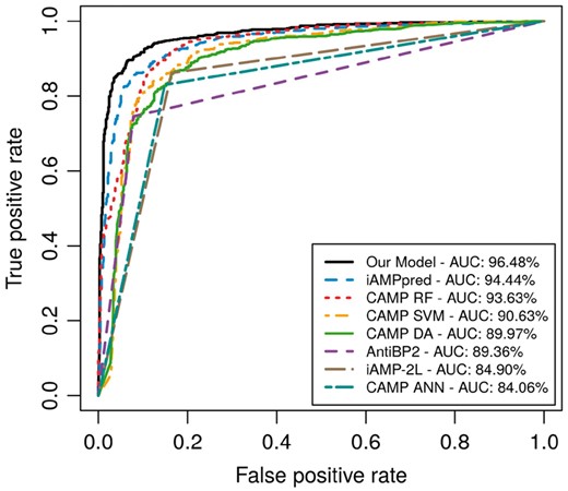
ROC curves are shown for the various methods compared, ordered from high to low performance in terms of area under the curve (AUC). Straight lines for AntiBP2, CAMP-ANN, and iAMP-2 L approximate the ROC curve using binary prediction results, as probability values are not provided. For the AntiBP2 curve, 211 testing sequences are excluded by the AntiBP2 server due to length restrictions set by the server

Comparative analysis showing our DNN to have better performance against the above AMP prediction servers on three additional datasets is provided in the Supplementary Information.

3.3 Reduced alphabet model analysis

A 2D t-SNE representation for the trained amino acid embedding vectors of our DNN production model (described in Section 2) is shown in Figure 3. Based on the proximity of neighboring amino acids in this representation, one can see that the DNN has learned basic amino acid physicochemical properties. Residues located closer together share more similar activation patterns, while more dissimilar amino acids are also farther in the projection. For example, the negative amino acids aspartic acid (D) and glutamic acid (E) are close to each other, and their distance from the padding character (X) may reflect the importance of charge in attracting AMPs to bacterial membranes (Boman, 2003; Wang, 2010). Amino acids with uncharged side chains, such as serine (S), threonine (T), asparagine (N) and glutamine (Q), are also neighbors. It is perhaps unsurprising to see amino acids with unique roles for structure formation or ligand interactions as slightly isolated and more distant. For example, cysteine (C), which forms disulfide bonds, stands on its own in the bottom right. Tryptophan (W), slightly separated on the right, has a preference for hydrophobic cores and a bulky indole side chain that is involved in aromatic stacking interactions (Betts and Russell, 2003).

Fig. 3.

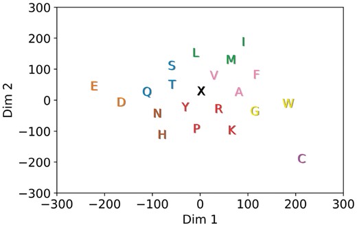
 A 2D t-SNE (Van der Maaten and Hinton, 2008) projection of the 128D amino acid embedding vectors. K-means was used to select clusters for the DNN-reduced alphabet as listed in Table S6 of the Supplementary Information

The coloring of the amino acids in Figure 3 denotes the 9 clusters (based on k-means) that can now be used to encode a peptide sequence in place of the classic amino acids and the padding ‘X’ letter. We evaluate whether this reduced encoding still retains enough information to recognize AMPs from non-AMPs. As described in Section 2, average ACC and MCC values (over 100 independent evaluations via our DNN model) and SD values are shown in row 10 in Table 2. Comparison with the DNN model operating on the full alphabet (of 21 letters) shows a slight drop of about 1.4% in ACC and 0.03 in MCC by the reduced alphabet. Despite using only 9 of the original 21 letters, the DNN-reduced model still outperforms all other non-DNN predictors listed in Table 2 in terms of ACC, MCC and auROC. Table 2 also shows that DNN-reduced alphabet confers good performance to gkmSVM as well (row 12). ACC and MCC scores are similarly reduced (compared to the full-size alphabet) by around 1.7% and 0.03, respectively. Evaluations using additional values for k are available in the Supplementary Information.

To ensure specific amino acid membership in clusters is playing a role and that a DNN would not perform just as well with randomly assigned clusters (randomly grouping amino acids into pseudo-amino acids), we generate 100 random alphabets (as described in Section 2) and evaluate them via our DNN model on the testing dataset. The performance of DNN models and the gkmSVM models on the random alphabets (averaged over the 100 runs), shown in rows 11 and 13 of Table 2, respectively, are the worst compared to all other methods in terms of SENS, ACC and MCC, suggesting cluster membership is important; the gkmSVM model on the random alphabets also yields the lowest ACC. A one-sided t-test reveals that the greater performance for the DNN-reduced alphabet DNN model over the random alphabet DNN models is statistically significant in terms of both ACC (P < 2.2 × ${10}^{-16}$⁠, df = 116.1, t = 24.8) and MCC (P < 2.2 × ${10}^{-16}$⁠, df = 112.3, t = 25.5). Similarly, a one-sided t-test reveals that the greater performance for the DNN-reduced alphabet gkmSVM model over the random alphabet gkmSVM models is statistically significant in terms of both ACC (P < 2.2 × ${10}^{-16}$⁠, df = 99, $t=-27.5$⁠) and MCC (P < 2.2 × ${10}^{-16}$⁠, df = 99, $t=-27.4$⁠).

4 Discussion

We have presented a new DNN-based classifier that achieves better AMP recognition performance compared to existing, state-of-the-art methods. To the best of our knowledge, this is the first time a deep learning approach has been applied to address AMP classification. By utilizing a deep network architecture, the proposed model automatically extracts expert-free features and so removes the reliance on domain experts for feature construction. The production model and all datasets are made available via the AMP Scanner web server that accompanies this paper. The production model can correctly identify over 98% of the AMPs listed as active against Gram-positive and/or Gram-negative bacteria currently available in the APD vr.3 and $\ge 10$ amino acid in length. The server supports high-throughput screening experiments to aid systematic virtual screenings of peptide libraries by wet-laboratory researchers. The reduced alphabet (of 9 letters) learned from the DNN model (additionally utilizing statistical techniques) further aids these efforts by reducing the size of the sequence space that can be considered when exploring for novel peptides with AMP activity. The DNN model on the reduced alphabet retains good AMP recognition accuracy, even outperforming other non-DNN methods operating on the full alphabet of 21 letters.

An open question in AMP research is how computational AMP predictions may relate to actual biological activity. Recent work by Lee et al. (2016) supports the notion that some models may predict more indirect properties. After comparing predictions on α-helical AMPs using an SVM and 12 physicochemical descriptors to small-angle X-ray scattering data, Lee et al. (2016) find that results best correlated with negative Gaussian membrane curvature. While results for the particular features used in (Lee et al., 2016) do not correlate with a more direct measure of AMP activity like minimum inhibitory concentration, disruption of bulk membrane properties (e.g. membrane curvature, lipid clustering, etc.) is a well-known mechanism of action for AMPs to kill bacteria and has been extensively studied in AMPs such as the human cathelicidin LL-37 (Epand et al., 2016).

It is possible that indirect AMP signatures are also being identified by the DNN model which relate more to their structural properties than direct measures of their antibacterial activity (such as minimum inhibitory concentration). Therefore, probabilities associated with model predictions ought to be limited to the context of recognizing AMP-like peptides within a list of one or more unknown sequences. In other words, the probabilities for two peptides predicted as ‘AMP’ should not be directly compared and interpreted as one having ‘stronger’ or ‘weaker’ antibacterial activity against any given bacteria. The availability of reliable direct measures of AMP activity on large AMP datasets will allow the field to proceed beyond binary classification to build models, DNN ones included, that directly predict antibacterial activity against specific species of bacteria.

Additional future work can consider different network architectures, such as variational encoders and/or generative adversarial networks, which have been shown highly effective in finding latent structures and features (Goodfellow et al., 2014; Kingma and Welling, 2014). More recent methods, such as Dynamic Memory Networks, which have seen great success in complex natural language-processing and speech recognition tasks, may also present appealing directions for further investigation (Kumar et al., 2016).

Acknowledgements

We thank the members of the NIAID BCBB and Shehu laboratories as well as Jianlin Cheng for helpful feedback and suggestions to improve this work.

Funding

This work was supported in part by National Science Foundation [1144106 to A.S.].

Conflict of Interest: none declared.