


Abstract
Genome-wide datasets produced for association studies have dramatically increased in size over the past few years, with modern datasets commonly including millions of variants measured in dozens of thousands of individuals. This increase in data size is a major challenge severely slowing down genomic analyses, leading to some software becoming obsolete and researchers having limited access to diverse analysis tools.
Here we present two R packages, bigstatsr and bigsnpr, allowing for the analysis of large scale genomic data to be performed within R. To address large data size, the packages use memory-mapping for accessing data matrices stored on disk instead of in RAM. To perform data pre-processing and data analysis, the packages integrate most of the tools that are commonly used, either through transparent system calls to existing software, or through updated or improved implementation of existing methods. In particular, the packages implement fast and accurate computations of principal component analysis and association studies, functions to remove single nucleotide polymorphisms in linkage disequilibrium and algorithms to learn polygenic risk scores on millions of single nucleotide polymorphisms. We illustrate applications of the two R packages by analyzing a case–control genomic dataset for celiac disease, performing an association study and computing polygenic risk scores. Finally, we demonstrate the scalability of the R packages by analyzing a simulated genome-wide dataset including 500 000 individuals and 1 million markers on a single desktop computer.
https://privefl.github.io/bigstatsr/ and https://privefl.github.io/bigsnpr/.
Supplementary data are available at Bioinformatics online.
1 Introduction
Genome-wide datasets produced for association studies have dramatically increased in size over the past few years, with modern datasets commonly including millions of variants measured in dozens of thousands of individuals. As a consequence, most existing software and algorithms have to be continuously optimized in order to avoid obsolescence. For computing principal component analysis (PCA), commonly performed to account for population stratification in association, a fast mode named FastPCA has been added to the software EIGENSOFT, and FlashPCA has been replaced by FlashPCA2 (Abraham and Inouye, 2014; Abraham et al., 2016; Galinsky et al., 2016; Price et al., 2006). PLINK 1.07, which has been a central tool in the analysis of genotype data, has been replaced by PLINK 1.9 to speed-up computations, and there is also an alpha version of PLINK 2.0 that will handle more data types (Chang et al., 2015; Purcell et al., 2007).
Increasing size of genetic datasets is a source of major computational challenges and many analytical tools would be restricted by the amount of memory (RAM) available on computers. This is particularly a burden for commonly used analysis languages such as R. For analyzing genotype datasets in R, a range of software are available, including for example the popular R packages GenABEL, SNPRelate and GWASTools (Aulchenko et al., 2007; Gogarten et al., 2012; Zheng et al., 2012b). Solving memory issues for languages such as R would give access to a broad range of already implemented tools for data analysis. Fortunately, strategies have been developed to avoid loading large datasets in RAM. For storing and accessing matrices, memory-mapping is very attractive because it is seamless and usually much faster to use than direct read or write operations. Storing large matrices on disk and accessing them via memory-mapping has been available for several years in R through ‘big.matrix’ objects implemented in the R package bigmemory (Kane et al., 2013).
2 Approach
In order to perform analyses of large-scale genomic data in R, we developed two R packages, bigstatsr and bigsnpr, that provide a wide-range of building blocks which are parts of standard analyses. R is a programming language that makes it easy to tie together existing or new functions to be used as part of large, interactive and reproducible analyses (R Core Team, 2017). We provide a similar format as filebacked ‘big.matrix’ objects that we called ‘Filebacked Big Matrices (FBMs)’. Thanks to this matrix-like format, algorithms in R/C++ can be developed or adapted for large genotype data. This data format is a particularly good trade-off between easiness of use and computation efficiency, making our code both simple and fast. Package bigstatsr implements many statistical tools for several types of FBMs (unsigned char, unsigned short, integer and double). This includes implementation of multivariate sparse linear models, PCA, association tests, matrix operations and numerical summaries. The statistical tools developed in bigstatsr can be used for other types of data as long as they can be represented as matrices. Package bigsnpr depends on bigstatsr, using a special type of filebacked big matrix (FBM) object to store the genotypes, called ‘FBM.code256’. Package bigsnpr implements algorithms which are specific to the analysis of single nucleotide polymorphism (SNP) arrays, such as calls to external software for processing steps, Input/Output (I/O) operations from binary PLINK files and data analysis operations on SNP data (thinning, testing, predicting and plotting). We use both a real case–control genomic dataset for celiac disease and large-scale simulated data to illustrate application of the two R packages, including two association studies and the computation of polygenic risk scores (PRS). We compare results from bigstatsr and bigsnpr with those obtained by using command-line software PLINK, EIGENSOFT and PRSice, and R packages SNPRelate and GWASTools. We report execution times along with the code to perform major computational tasks. For a comprehensive comparison between R packages bigstatsr and bigmemory, see Supplementary notebook ‘bigstatsr-and-bigmemory’.
3 Materials and methods
3.1 Memory-mapped files
The two R packages do not use standard read operations on a file nor load the genotype matrix entirely in memory. They use a hybrid solution: memory-mapping. Memory-mapping is used to access data, possibly stored on disk, as if it were in memory. This solution is made available within R through the BH package, providing access to Boost C++ Header Files (http://www.boost.org/).
We are aware of the software library SNPFile that uses memory-mapped files to store and efficiently access genotype data, coded in C++ (Nielsen and Mailund, 2008) and of the R package BEDMatrix (https://github.com/QuantGen/BEDMatrix) which provides memory-mapping directly for binary PLINK files. With the two packages we developed, we made this solution available in R and in C++ via package Rcpp (Eddelbuettel and François, 2011). The major advantage of manipulating genotype data within R, almost as if it were a standard matrix in memory, is the possibility of using most of the other tools that have been developed in R (R Core Team, 2017). For example, we provide sparse multivariate linear models and an efficient algorithm for PCA based on adaptations from R packages biglasso and RSpectra (Qiu and Mei, 2016; Zeng and Breheny, 2017).
Memory-mapping provides transparent and faster access than standard read/write operations. When an element is needed, a small chunk of the genotype matrix, containing this element, is accessed in memory. When the system needs more memory, some chunks of the matrix are freed from the memory in order to make space for others. All this is managed by the operating system so that it is seamless and efficient. It means that if the same chunks of data are used repeatedly, it will be very fast the second time they are accessed, the third time and so on. Of course, if the memory size of the computer is larger than the size of the dataset, the file could fit entirely in memory and every second access would be fast.
3.2 Data management, pre-processing and imputation
We developed a special FBM object, called ‘FBM.code256’, that can be used to seamlessly store up to 256 arbitrary different values, while having a relatively efficient storage. Indeed, each element is stored in one byte which requires eight times less disk storage than double-precision numbers but four times more space than the binary PLINK format ‘.bed’ which can store only genotype calls. With these 256 values, the matrix can store genotype calls and missing values (four values), best guess genotypes (three values) and genotype dosages (likelihoods) rounded to two decimal places (201 values). So, we use a single data format that can store both genotype calls and dosages.
For pre-processing steps, PLINK is a widely-used software. For the sake of reproducibility, one could use PLINK directly from R via systems calls. We therefore provide wrappers as R functions that use system calls to PLINK for conversion and quality control and a variety of formats can be used as input (e.g. vcf, bed/bim/fam, ped/map) and bed/bim/fam files as output (Supplementary Fig. S1). Package bigsnpr provides fast conversions between bed/bim/fam PLINK files and the ‘bigSNP’ object, which contains the genotype FBM (FBM.code256), a data frame with information on samples and another data frame with information on SNPs. We also provide another function which could be used to read from tabular-like text files in order to create a genotype in the format ‘FBM’. Finally, we provide two methods for converting dosage data to the format ‘bigSNP’ (Supplementary notebook ‘dosage’).
Most modern SNP chips provide genotype data with large call-rates. For example, the celiac data we use in this paper presents only 0.04% of missing values after quality control. Yet, most of the functions in bigstatsr and bigsnpr do not handle missing values. So, we provide two functions for imputing missing values of genotyped SNPs. Note that we do not impute completely missing SNPs which would require the use of reference panels and could be performed via e.g. imputation servers for human data (McCarthy et al., 2016). The first function is a wrapper to PLINK and Beagle (Browning and Browning, 2007) which takes bed files as input and return bed files without missing values, and should therefore be used before reading the data in R (Supplementary Fig. S2). The second function is a new algorithm we developed in order to have a fast imputation method without losing much of imputation accuracy. This function also provides an estimator of the imputation error rate by SNP for post-quality control. This algorithm is based on machine learning approaches for genetic imputation (Wang et al., 2012) and does not use phasing, thus allowing for a dramatic decrease in computation time. It only relies on some local XGBoost models (Chen and Guestrin, 2016). XGBoost, which is available in R, builds decision trees that can detect non-linear interactions, partially reconstructing phase, making it well suited for imputing genotype matrices. Our algorithm is the following: for each SNP, we divide the individuals in the ones which have a missing genotype (test set) and the ones which have a non-missing genotype for this particular SNP. Those latter individuals are further separated in a training set and a validation set (e.g. 80% training and 20% validation). The training set is used to build the XGBoost model for predicting missing data. The prediction model is then evaluated on the validation set for which we know the true genotype values, providing an estimator of the number of genotypes that have been wrongly imputed for that particular SNP. The prediction model is also projected on the test set (missing values) in order to impute them.
3.3 Population structure and SNP thinning based on linkage disequilibrium
For computing principal components (PCs) of a large-scale genotype matrix, we provide several functions related to SNP thinning and two functions for computing a partial singular value decomposition (SVD), one based on eigenvalue decomposition and the other one based on randomized projections, respectively named big_SVD and big_randomSVD (Fig. 1). While the function based on eigenvalue decomposition is at least quadratic in the smallest dimension, the function based on randomized projections runs in linear time in all dimensions (Lehoucq and Sorensen, 1996). Package bigstatsr uses the same PCA algorithm as FlashPCA2 called implicitly restarted Arnoldi method (IRAM), which is implemented in R package RSpectra. The main difference between the two implementations is that FlashPCA2 computes vector-matrix multiplications with the genotype matrix based on the binary PLINK file whereas bigstatsr computes these multiplications based on the FBM format, which enables parallel computations and easier subsetting.
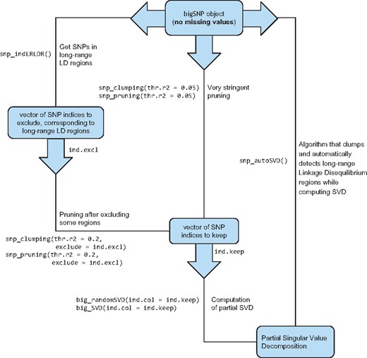
Functions available in packages bigstatsr and bigsnpr for the computation of a partial singular value decomposition of a genotype array, with three different methods for thinning SNPs
SNP thinning improves ascertainment of population structure with PCA (Abdellaoui et al., 2013). There are at least three different approaches to thin SNPs based on linkage disequilibrium. Two of them, named pruning and clumping, address SNPs in LD close to each other’s because of recombination events, while the third one address long-range regions with a complex LD pattern due to other biological events such as inversions (Price et al., 2008). First, pruning is an algorithm that sequentially scan the genome for nearby SNPs in LD, performing pairwise thinning based on a given threshold of correlation. Clumping is useful if a statistic is available for sorting the SNPs by importance. Clumping is usually used to post-process results of genome-wide association studies (GWAS) in order to keep only the most significant SNP per region of the genome. For PCA, the thinning procedure should remain unsupervised (no phenotype must be used) and we therefore propose to use the minor allele frequency (MAF) as the statistic of importance. This choice is consistent with the pruning algorithm of PLINK; when two nearby SNPs are correlated, PLINK keeps only the one with the highest MAF. Yet, in some worst-case scenario, the pruning algorithm can leave regions of the genome without any representative SNP at all (Supplementary notebook ‘pruning-vs-clumping’). So, we suggest to use clumping instead of pruning, using the MAF as the statistic of importance, which is the default in function snp_clumping of package bigsnpr. In practice, for the three datasets we considered, the clumping algorithm with the MAF provides similar sets of SNPs as when using the pruning algorithm (results not shown).
The third approach, which is generally combined with pruning, consists of removing SNPs in long-range LD regions (Price et al., 2008). Long-range LD regions for the human genome are available as an online table (https://goo.gl/8TngVE) that package bigsnpr can use to discard SNPs in these regions before computing PCs. However, the pattern of LD might be population specific, so we developed an iterative algorithm that automatically detects these long-range LD regions and removes them. This algorithm consists in the following steps: first, PCA is performed using a subset of SNP remaining after clumping (with MAFs), then outliers SNPs are detected using the robust Mahalanobis distance as implemented in method pcadapt (Luu et al., 2017). Finally, the algorithm considers that consecutive outlier SNPs are in long-range LD regions. Indeed, a long-range LD region would cause SNPs in this region to have strong consecutive weights (loadings) in the PCA. This algorithm is implemented in function snp_autoSVD of package bigsnpr and will be referred by this name in the rest of the paper.
3.4 Association tests and polygenic risk scores
The R packages also implement functions for computing PRS using two methods. The first method is the widely-used ‘Clumping + Thresholding’ (C + T, also called ‘Pruning + Thresholding’ in the literature) model based on univariate GWAS summary statistics as described in previous equations. Under the C + T model, a coefficient of regression is learned independently for each SNP along with a corresponding P-value (the GWAS part). The SNPs are first clumped (C) so that there remains only SNPs that are weakly correlated with each other. Thresholding (T) consists in removing SNPs that are under a certain level of significance (P-value threshold to be determined). A PRS is defined as the sum of allele counts of the remaining SNPs weighted by the corresponding regression coefficients (Chatterjee et al., 2013; Dudbridge, 2013; Euesden et al., 2015). On the contrary, the second approach does not use univariate summary statistics but instead train a multivariate model on all the SNPs and covariables at once, optimally accounting for correlation between predictors (Abraham et al., 2012). The currently available models are very fast sparse linear and logistic regressions. These models include lasso and elastic-net regularizations, which reduce the number of predictors (SNPs) included in the predictive models (Friedman et al., 2010; Tibshirani, 1996; Zou and Hastie, 2005). Package bigstatsr provides a fast implementation of these models by using efficient rules to discard most of the predictors (Tibshirani et al., 2012). The implementation of these algorithms is based on modified versions of functions available in the R package biglasso (Zeng and Breheny, 2017). These modifications allow to include covariates in the models, to use these algorithms on the special type of FBM called ‘FBM.code256’ used in bigsnpr and to remove the need of choosing the regularization parameter.
3.5 Data analyzed
In this paper, two datasets are analyzed: the celiac disease cohort and POPRES (Dubois et al., 2010; Nelson et al., 2008). The celiac dataset is composed of 15 283 individuals of European ancestry genotyped on 295 453 SNPs. The POPRES dataset is composed of 1385 individuals of European ancestry genotyped on 447 245 SNPs. For computation time comparisons, we replicated individuals in the celiac dataset 5 and 10 times in order to increase sample size while keeping the same eigen decomposition (up to a constant) and pairwise SNP correlations as the original dataset. To assess scalability of the packages for a biobank-scale genotype dataset, we formed another dataset of 500 000 individuals and 1 million SNPs, also through replication of the celiac dataset.
3.6 Reproducibility
All the code used in this paper along with results, such as execution times and figures, are available as HTML R notebooks in the Supplementary materials. In Supplementary notebook ‘public-data’, we provide some open-access data of domestic dogs so that users can test our code and functions on a moderate size dataset with 4342 samples and 145 596 SNPs (Hayward et al., 2016).
4 Results
4.1 Overview
We present the results of four different analyses. First, we illustrate the application of R packages bigstatsr and bigsnpr. Second, by performing two GWAS, we compare the performance of bigstatsr and bigsnpr to the performance obtained with FastPCA (EIGENSOFT 6.1.4) and PLINK 1.9, and also two R packages SNPRelate and GWASTools (Chang et al., 2015; Galinsky et al., 2016; Gogarten et al., 2012; Zheng et al., 2012b). PCA is a computationally intensive step of the GWAS, so that we further compare PCA methods on larger datasets. Third, by performing a PRS analysis with summary statistics, we compare the performance of bigstatsr and bigsnpr to the performance obtained with PRSice-2 (Euesden et al., 2015). Finally, we present results of the two new methods implemented in bigsnpr, one method for the automatic detection and removal of long-range LD regions in PCA and another for the in-sample imputation of missing genotypes (i.e. for genotyped SNPs only). We compare performance on two computers, a desktop computer with 64 GB of RAM and 12 cores (six physical cores), and a laptop with only 8 GB of RAM and 4 cores (two physical cores). For the functions that enable parallelism, we use half of the cores available on the corresponding computer. We present a table summarizing the features of different software in Supplementary Table S5.
4.2 Application
The data were pre-processed following steps from Supplementary Figure S1, removing individuals and SNPs with more than 5% of missing values, non-autosomal SNPs, SNPs with a MAF lower than 0.05 or a P-value for the Hardy–Weinberg exact test lower than 10−10, and finally, removing the first individual in each pair of individuals with a proportion of alleles shared IBD >0.08 (Purcell et al., 2007). For the POPRES dataset, this resulted in 1382 individuals and 344 614 SNPs with no missing value. For the celiac dataset, this resulted in 15 155 individuals and 281 122 SNPs with an overall genotyping rate of 99.96%. The 0.04% missing genotype values were imputed with the XGBoost method. If we would have used a standard R matrix to store the genotypes, this data would have required 32 GB of memory. On the disk, the ‘.bed’ file requires 1 GB and the ‘.bk’ file (storing the FBM) requires 4 GB.
We used bigstatsr and bigsnpr R functions to compute the first PCs of the celiac genotype matrix and to visualize them (Fig. 2). We then performed a GWAS investigating how SNPs are associated with celiac disease, while adjusting for PCs, and plotted the results as a Manhattan plot (Fig. 3). As illustrated in the Supplementary data, the whole pipeline is user-friendly, requires only 20 lines of R code and there is no need to write temporary files or objects because functions of packages bigstatsr and bigsnpr have parameters which enable subsetting of the genotype matrix without having to copy it.
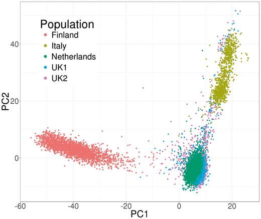
Principal components of the celiac cohort genotype matrix produced by package bigstatsr
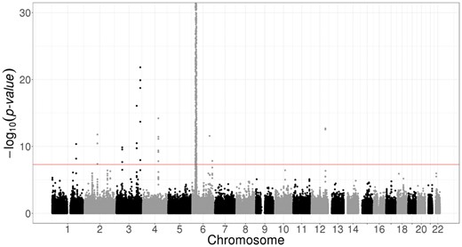
Manhattan plot of the celiac disease cohort produced by package bigsnpr. Some SNPs in chromosome 6 have P-values smaller than the 10−30 threshold used for visualization purposes
To illustrate the scalability of the two R packages, we performed a GWAS analysis on 500 K individuals and 1 M SNPs. The GWAS analysis completed in ∼11 h using the aforementioned desktop computer. The GWAS analysis was composed of four main steps. First we converted binary PLINK files in the format ‘bigSNP’ in 1 h. Then, we removed SNPs in long-range LD regions and used SNP clumping, leaving 93 083 SNPs in 5.4 h. Then, the 10 first PCs were computed on the 500 K individuals and these remaining SNPs in 1.8 h. Finally, we performed a linear association test on the complete 500 K dataset for each of the 1 M SNPs, using the 10 first PCs as covariables in 2.9 h.
4.3 Performance and precision comparisons
First, we compared the GWAS computations obtained with bigstatsr and bigsnpr to the ones obtained with PLINK 1.9 and EIGENSOFT 6.1.4, and also two R packages SNPRelate and GWASTools. For most functions, multithreading is not available yet in PLINK, nevertheless, PLINK-specific algorithms that use bitwise parallelism (e.g. pruning) are still faster than the parallel algorithms reimplemented in package bigsnpr (Table 1). Overall, performing a GWAS on a binary outcome with bigstatsr and bigsnpr is as fast as when using EIGENSOFT and PLINK, and 19–45 times faster than when using R packages SNPRelate and GWASTools. For performing an association study on a continuous outcome, we report a dramatic increase in performance by using bigstatsr and bigsnpr, making it possible to perform such analysis in <2 min for a relatively large dataset such as the celiac dataset. This analysis was 7–19 times faster as compared to PLINK 1.9 and 28–74 times faster as compared to SNPRelate and GWASTools (Table 1). Note that the PC scores obtained are more accurate as compared to PLINK (see the last paragraph of this subsection), which is also the case for the P-values computed for the two GWAS (see Supplementary notebook ‘GWAS-comparison’).
Execution times with bigstatsr and bigsnpr compared to PLINK 1.9 and FastPCA (EIGENSOFT) and also to R packages SNPRelate and GWASTools for making a GWAS for the celiac dataset (15 155 individuals and 281 122 SNPs). The first execution time is with a desktop computer (6 cores used and 64 GB of RAM) and the second one is with a laptop (2 cores used and 8 GB of RAM)
| Operation\software | Execution times (in seconds) | ||
|---|---|---|---|
| FastPCA | bigstatsr | SNPRelate | |
| PLINK 1.9 | bigsnpr | GWASTools | |
| Converting PLINK files | n/a | 6/20 | 13/33 |
| Pruning | 4/4 | 14/52 | 33/32 |
| Computing 10 PCs | 305/314 | 58/183 | 323/535 |
| GWAS (binary phenotype) | 337/284 | 291/682 | 16 220/17 425 |
| GWAS (continuous phenotype) | 1348/1633 | 10/23 | 6115/7101 |
| Total (binary) | 646/602 | 369/937 | 16 589/18 025 |
| Total (continuous) | 1657/1951 | 88/278 | 6484/7701 |
Second, we compared the PRS analysis performed with the R packages to the one using PRSice-2. There are five main steps in such an analysis (Table 2), including four steps handled with functions of packages bigstatsr and bigsnpr. The remaining step is the reading of summary statistics which can be performed with the widely used function fread of R package data.table. Using bigstatsr and bigsnpr results in an analysis as fast as with PRSice-2 when using our desktop computer, and three times slower when using our laptop (Table 2).
Execution times with bigstatsr and bigsnpr compared to PRSice for making a PRS on the celiac dataset based on summary statistics for height. The first execution time is with a desktop computer (6 cores used and 64 GB of RAM) and the second one is with a laptop (2 cores used and 8 GB of RAM)
| Operation\software | Execution times (in seconds) | |
|---|---|---|
| PRSice | bigstatsr and bigsnpr | |
| Converting PLINK files | — | 6/20 |
| Reading summary stats | — | 4/6 |
| Clumping | — | 9/31 |
| PRS | — | 2/33 |
| Compute P-values | — | 1/1 |
| Total | 22/29 | 22/91 |
| Operation\software | Execution times (in seconds) | |
|---|---|---|
| PRSice | bigstatsr and bigsnpr | |
| Converting PLINK files | — | 6/20 |
| Reading summary stats | — | 4/6 |
| Clumping | — | 9/31 |
| PRS | — | 2/33 |
| Compute P-values | — | 1/1 |
| Total | 22/29 | 22/91 |
Finally, on our desktop computer, we compared the computation times of FastPCA (fast mode of EIGENSOFT), FlashPCA2 and PLINK 2.0 (approx mode) to the similar function big_randomSVD implemented in bigstatsr. For each comparison, we used the 93 083 SNPs which were remaining after pruning and we computed 10 PCs. We used the datasets of growing size simulated from the celiac dataset (from 15 155 to 151 550 individuals). Overall, function big_randomSVD is almost twice as fast as FastPCA and FlashPCA2 and eight times as fast as when using parallelism with six cores, an option not currently available in either FastPCA or FlashPCA2 (Fig. 4). PLINK 2.0 is faster than bigstatsr with a decrease in time of 20–40%. We also compared results in terms of precision by comparing squared correlation between approximated PCs and ‘true’ PCs provided by an exact eigen decomposition obtained with PLINK 2.0 (exact mode). Package bigstatsr and FlashPCA2 (that use the same algorithm) infer all PCs with a squared correlation of more than 0.999 between true PCs and approximated ones (Fig. 5). Yet, FastPCA (fast mode of EIGENSOFT) and PLINK 2.0 (that use the same algorithm) infer the true first six PCs but the squared correlation between true PCs and approximated ones decreases for further PCs (Fig. 5).
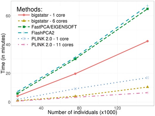
Benchmark comparisons between randomized partial singular value decomposition available in FlashPCA2, FastPCA (fast mode of SmartPCA/EIGENSOFT), PLINK 2.0 (approx mode) and package bigstatsr. It shows the computation time in minutes as a function of the number of samples. The first 10 principal components have been computed based on the 93 083 SNPs which remained after thinning
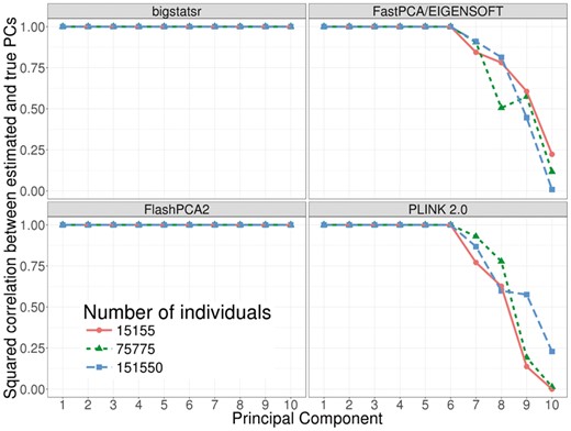
Precision comparisons between randomized partial singular value decomposition available in FlashPCA2, FastPCA (fast mode of SmartPCA/EIGENSOFT), PLINK 2.0 (approx mode) and package bigstatsr. It shows the squared correlation between approximated PCs and ‘true’ PCs (produced by the exact mode of PLINK 2.0) of the celiac dataset (whose individuals have been repeated 1, 5 and 10 times)
4.4 Automatic detection of long-range LD regions
For detecting long-range LD regions during the computation of PCA, we tested the function snp_autoSVD on both the celiac and POPRES datasets. For the POPRES dataset, the algorithm converged in two iterations. The first iterations found three long-range LD regions in chromosomes 2, 6 and 8 (Supplementary Table S1). We compared the PCs of genotypes obtained after applying snp_autoSVD with the PCs obtained after removing pre-determined long-range LD regions (https://goo.gl/8TngVE) and found a mean correlation of 89.6% between PCs, mainly due to a rotation of PC7 and PC8 (Supplementary Table S2). For the celiac dataset, we found five long-range LD regions (Supplementary Table S3) and a mean correlation of 98.6% between PCs obtained with snp_autoSVD and the ones obtained by clumping and removing pre-determined long-range LD regions (Supplementary Table S4).
For the celiac dataset, we further compared results of PCA obtained when using snp_autoSVD and when computing PCA without removing any long range LD region (only clumping at R2 > 0.2). When not removing any long range LD region, we show that PC4 and PC5 do not capture population structure and correspond to a long-range LD region in chromosome 8 (Supplementary Figs S3 and S4). When automatically removing some long-range LD regions with snp_autoSVD, we show that PC4 and PC5 reflect population structure (Supplementary Fig. S3). Moreover, loadings are more equally distributed among SNPs after removal of long-range LD regions (Supplementary Fig. S4). This is confirmed by Gini coefficients (measure of dispersion) of each squared loadings that are significantly smaller when computing PCA with snp_autoSVD than when no long-range LD region is removed (Supplementary Fig. S5).
4.5 Imputation of missing values for genotyped SNPs
For the imputation method based on XGBoost, we compared the imputation accuracy and computation times with Beagle on the POPRES dataset (with no missing value). The histogram of the MAFs of this dataset is provided in Supplementary Figure S6. We used a beta-binomial distribution to simulate the number of missing values by SNP and then randomly introduced missing values according to these numbers, resulting in ∼3% of missing values overall (Supplementary Fig. S7). Imputation was compared between function snp_fastImpute of package bigsnpr and Beagle 4.1 (version of January 21, 2017) by counting the percentage of imputation errors (when the imputed genotype is different from the true genotype). Overall, in three runs, snp_fastImpute made only 4.7% of imputation errors and Beagle made only 3.1% of errors. Yet, it took Beagle 14.6 h to complete while snp_fastImpute only took 42 min (20 times less). We also note that snp_fastImpute made less 0/2 switching errors, i.e. imputing with a homozygous referent where the true genotype is a homozygous variant, or the contrary (Supplementary notebook ‘imputation’). We also show that the estimation of the number of imputation errors provided by function snp_fastImpute is accurate (Supplementary Fig. S8), which can be useful for post-processing the imputation by removing SNPs with too many errors (Supplementary Fig. S9). For the celiac dataset in which there were already missing values, in order to further compare computation times, we report that snp_fastImpute took <10 h to complete for the whole genome whereas Beagle did not finish imputing chromosome 1 in 48 h.
5 Discussion
We have developed two R packages, bigstatsr and bigsnpr, which enable multiple analyses of large-scale genotype datasets in R thanks to memory-mapping. Linkage disequilibrium pruning, PCA, association tests and computation of PRS are made available in these software. Implemented algorithms are both fast and memory-efficient, allowing the use of laptops or desktop computers to make genome-wide analyses. Technically, bigstatsr and bigsnpr could handle any size of datasets. However, if the OS has to often swap between the file and the memory for accessing the data, this would slow down data analysis. For example, the PCA algorithm in bigstatsr is iterative so that the matrix has to be sequentially accessed over a hundred times. If the number of samples times the number of SNPs remaining after pruning is larger than the available memory, this slowdown would happen. For instance, a 32 GB computer would be slow when computing PCs on more than 100K samples and 300K SNPs remaining after LD thinning.
The two R packages use a matrix-like format, which makes it easy to develop new functions in order to experiment and develop new ideas. Integration in R makes it possible to take advantage of the vast and diverse R libraries. For example, we developed a fast and accurate imputation algorithm for genotyped SNPs using the widely-used machine learning algorithm XGBoost available in the R package xgboost. Other functions, not presented here, are also available and all the functions available within the package bigstatsr are not specific to SNP arrays, so that they could be used for other omic data or in other fields of research.
We think that the two R packages and the corresponding data format could help researchers to develop new ideas and algorithms to analyze genome-wide data. For example, we wish to use these packages to train much more accurate predictive models than the standard C + T model currently in use for computing PRS. As a second example, multiple imputation has been shown to be a very promising method for increasing statistical power of a GWAS (Palmer and Pe’er, 2016), and it could be implemented with the data format ‘FBM.code256’ without having to write multiple files.
Funding
Authors acknowledge LabEx PERSYVAL-Lab (ANR-11-LABX-0025-01). Authors also acknowledge the Grenoble Alpes Data Institute that is supported by the French National Research Agency under the ‘Investissements d’avenir’ program (ANR-15-IDEX-02).
Acknowledgements
Authors would like to thank the reviewers of this paper because their comments and suggestions have led to a significant improvement of this paper.
Conflict of Interest: none declared.
References

