Leveraging known genomic variants to improve detection of variants, especially close-by Indels

Abstract

Motivation

The detection of genomic variants has great significance in genomics, bioinformatics, biomedical research and its applications. However, despite a lot of effort, Indels and structural variants are still under-characterized compared to SNPs. Current approaches based on next-generation sequencing data usually require large numbers of reads (high coverage) to be able to detect such types of variants accurately. However Indels, especially those close to each other, are still hard to detect accurately.

Results

We introduce a novel approach that leverages known variant information, e.g. provided by dbSNP, dbVar, ExAC or the 1000 Genomes Project, to improve sensitivity of detecting variants, especially close-by Indels. In our approach, the standard reference genome and the known variants are combined to build a meta-reference, which is expected to be probabilistically closer to the subject genomes than the standard reference. An alignment algorithm, which can take into account known variant information, is developed to accurately align reads to the meta-reference. This strategy resulted in accurate alignment and variant calling even with low coverage data. We showed that compared to popular methods such as GATK and SAMtools, our method significantly improves the sensitivity of detecting variants, especially Indels that are close to each other. In particular, our method was able to call these close-by Indels at a 15–20% higher sensitivity than other methods at low coverage, and still get 1–5% higher sensitivity at high coverage, at competitive precision. These results were validated using simulated data with variant profiles extracted from the 1000 Genomes Project data, and real data from the Illumina Platinum Genomes Project and ExAC database. Our finding suggests that by incorporating known variant information in an appropriate manner, sensitive variant calling is possible at a low cost.

Availability and implementation

Implementation can be found in our public code repository https://github.com/namsyvo/IVC.

Supplementary information

Supplementary data are available at Bioinformatics online.

1 Introduction

The detection of genomic variants has great significance in genomics, bioinformatics, biomedical research and its applications (1000 Genomes Project Consortium, 2012, 2015; Pabinger et al., 2014). Recent advances in next-generation sequencing (NGS) technologies make it possible to provide cost-effective, high-throughput and large-scale sequencing data for humans and other species (Auton et al., 2012; Lek et al., 2016). This facilitates a wide range of genomics and bioinformatics research including genomic variant detection. Many algorithms and tools with several approaches have been developed for calling genomic variants including SNPs, Indels and Structural Variants. Most of them are based on statistical methods such as Bayesian methods, Hidden Markov models or logistic regression models (Bansal et al., 2010; Challis et al., 2012; Chen et al., 2009; DePristo et al., 2011; Garrison and Marth, 2012; Li, 2011; Mose et al., 2014; Wang et al., 2013; Ye et al., 2009). Although these methods are well-established, they still suffer from detecting Indels and structural variants in repetitive or densely altered regions of the genome. Li (2014) has shown that Indels that are close to each other (close-by Indels) can make it challenging for aligners to get the correct alignments and consequently for variant callers to make the correct calls. Recently, Jiang et al. (2015) have shown that Indels are more abundant than currently appreciated. Furthermore, Chaisson et al. (2014), by analyzing a haploid human genome (CHM1) using single-molecule, real-time DNA sequencing, have detected several folds more Indels than previously reported. Missing these variants can lead to inaccurate downstream analyses such as characterizing tumor evolution or predicting therapeutic responses. Therefore, there is still need for improving sensitivity of Indel detection.

Most of the current variant calling methods detect variants based on analyzing aligned reads from external aligners (Pabinger et al., 2014). To speed up the alignment process, most aligners ignore the interdependency between reads coming from the same regions, which might produce inconsistent aligned reads and therefore complicate variant calling (Li, 2014). Researchers usually perform realignment to recover misaligned reads at the region of interests (Albers et al., 2011; DePristo et al., 2011). Some methods perform local assembly to construct unitigs, and then map the unitigs against the reference genome to call variants (Carnevali et al., 2012; Mose et al., 2014). Some other methods exploit a special data structure called alignment graphs to improve detection of long Indels (Marschall et al., 2013). Researchers also exploit multi-samples to support variant detection (Bansal et al., 2010; Li, 2011; Wang et al., 2013). Nevertheless, they still have not taken full advantage of input data to support variant calling process. Consequently, they usually require high sequencing coverage to be able to detect variants accurately.

Currently, a large number of genomic variants in populations of humans and other species have been collected in public databases. For example, a lot of human genomic variants are detected from a large number of individuals with a lot of effort such as dbSNP (Wheeler et al., 2007), dbVar and DGVa (Lappalainen et al., 2013), 1000 Genomes Project (1000 Genomes Project Consortium, 2015) or ExAC (Lek et al., 2016). Therefore it would be desirable to design methods which can efficiently exploit them to support calling variants in new genomes. For this purpose, SOAPsnp (Li et al., 2009b) calculates a prior-genotype probability by the use of dbSNP in the analysis of human data; while Atlas (Shen et al., 2010) uses prior SNP probability and prior error probability in its training datasets. Nevertheless, those methods have not exploited known variant information efficiently to support variant calling. In particular, these tools have not used that known variants to support analyzing aligned reads. Recently, BWBBLE (Huang et al., 2013) is among a few tools which can use known variants to support read alignment, but this method has not been adapted to variant calling problem.

In this paper, we introduce a novel method that leverages known variant information to detect both known and unknown genomic variants from NGS data, especially close-by Indels. In this method we combine reference genomes and their associated known variant profiles in an appropriate manner to help perform read alignment and variant calling efficiently and accurately. We then develop an algorithm, which can take into account known variant information, for alignment of reads to the reference. This strategy allows reads to be aligned more accurately, and variants can be called more accurately even with few numbers of reads (low coverage) compared to conventional methods. In particular, our method is better at calling Indels that are otherwise hard to call even at high coverage. The method’s high accuracy at low coverage can help reduce experimental cost of variant detection.

2 Materials and methods

The overall objective of our method is to detect genomic variants from short reads that come from an individual’s genome. Our method incorporates known information of genomic variants, which are collected in public databases by efforts such as the 1000 Genomes Project or ExAC, into the variant calling process. We expect that information of known variants can help to identify the known variants of a new individual’s genome more efficiently. More importantly, we also expect that by leveraging the known information in the variant calling process, we can detect unknown variants, i.e. variants that do not exist in databases, more accurately.

Our method, called IVC (Integrated Variant Calling), includes two main contributions: (i) a meta-genome representation which combines the reference genome and known variant profile in an appropriate manner, and (ii) a known-variant-sensitive alignment algorithm which can take into account known variants in determining optimal alignment. Both of them are designed to efficiently and effectively exploit known variants in read alignment and variant detection processes, which is difficult to do with standard reference genomes and conventional alignment algorithms. Two other techniques are also introduced: (iii) an iterated randomized algorithm which can find seeds efficiently, and (iv) a strategy to update variant profiles during the alignment process, which turns out can help improve accuracy of read alignment and therefore the variant calling. These contributions will be described in the following sections.

2.1 Representing and indexing reference genomes with incorporated known genomic variants

Many methods of calling variants depend on the alignment of short reads to a reference genome. To incorporate genomic variants into the reference genome, several approaches have been proposed such as graph representations for multiple genomes (Schneeberger et al., 2009), strings with wildcards (Thachuk, 2011) or strings with IUPAC symbols (Huang et al., 2013). While these approaches are theoretically interesting, they either cannot fully describe variants or are computationally inefficient or difficult to implement in practice.

Here we introduce a novel representation which incorporates variants into the reference genome in a simpler and more efficient way. First, we create a reference meta-genome M which is composed of characters A, C, G, T, N and V. Positions with A, C, G, T and N are corresponding to bases in the standard reference genome which are not marked as variant locations in the databases. Positions with V represent locations of known genomic variants in databases, which can be either SNPs or Indels (other types of variants will be added into the design in the future). Thus, a V character can represent multiple bases (e.g. A or C) in case of SNPs or multiple sequences of bases (e.g. AC or ACGGT) in case of Indels. Together with this reference meta-genome, we create a hash table H with keys representing locations of known variants and values representing the variant profiles at corresponding locations. During the alignment of short reads to the reference, whenever a known variant location is reached, the hash table is used to retrieve variants at that location. The main advantage of using a hash table is that it allows us to retrieve information of known variants in a quick and simple way, although it might require accessing both data structures.

Together with the meta-genome M and the hash table H, an index I is also created to speed up the alignment of short reads to the reference. The use of an index to facilitate short-read alignment is commonplace. The purpose of such indexes is to quickly identify long common substrings, known as seeds, between reads and the reference. Those seeds are then extended to find the complete alignment between reads and the reference. Researchers have used various types of data structures such as hash tables or FM-indexes to build such indexes (Li and Homer, 2010). A standard FM-index is a data structure built for a specific string to allow optimal linear storage and linear time substring query on that string (Ferragina and Manzini, 2005). In particular, given a string s, to find out if s is a substring of another string t, the FM-index search algorithm starts at the end of s and proceeds in a backward fashion to identify all currently matched suffixes of s in t, using the FM-index data structure created from t. The search stops when either it cannot find any occurrences of the current suffix of s in t or it reaches beyond the beginning of s.

In our method, we exploit the FM-index for indexing the meta-genome M, which consists of characters A, C, G, T, N and V as described above, in which V is considered as a wildcard character. However, to facilitate alignment of reads to the reference meta-genome, we developed an iterated randomized algorithm to replace the traditional FM-index search algorithm. This algorithm turns out to be very efficient in our experiments as described in next sections.

2.2 Aligning reads to the reference meta-genome

The purpose of aligning reads to the reference meta-genome in our method is to keep track of genomic differences between reads and the reference. Our alignment strategy is similar to popular methods in its decomposition of the alignment process into two steps:

1. (Seeding phase) Searching for (appropriate) seeds of the alignment between reads and the reference meta-genome.

2. (Extension phase) Seeds are extended on both sides (left and right) on reads and on the reference into a complete alignment.

However, to improve accuracy of read alignment, in each phase we introduce several novel techniques as described in the following.

2.2.1 Seeding phase

Many current alignment methods determine proper seeds based on long exact matches between reads and the reference genome. A good strategy to determine long exact matches must not start near positions on reads that contain differences between reads and the reference. However, these differences can occur at any positions on reads. Thus, several seed finding methods such as CUSHAW2 (Liu and Schmidt, 2012) are essentially brute-force, which are computationally expensive.

Our seed finding strategy is an iterated randomized algorithm, which is faster than the brute-force algorithm while still having competitive accuracy. A more detailed analysis of this strategy is given in Supplementary Material. Basically, our seed finding algorithm is based on searching for exact substrings on an FM index with the following modifications:

1. The search for seeds starts at a random position in r and proceeds in a forward fashion. Instead of considering all positions on the read in the brute-force manner to find the longest exact matches, this algorithm starts the search from a random position on the read. By repeating this several times, we can find the near longest exact matches after a number of random iterations which is much less than those numbers required by the brute-force manner (Vo et al., 2014). The algorithm also performs forward search from a position near the beginning of the read than the conventional backward search from the end of the read. The main advantage of doing this is making the search less likely encountering sequencing errors. This is based on the observation that probabilities of sequencing errors are likely increased from the beginning to the end of the reads (Wang et al., 2012).

2. The search for seeds ends as either it reaches a known variant location, or it cannot find any occurrences of the current suffix of r in M, or it reaches beyond the end of r. To avoid as many as possible variant locations (one source of differences between reads and the reference) as searching for seeds, here we exploit one advantage of the meta-genome representation. By looking at V characters on the meta-genome M using the hash table H, we can stop the search for seeds whenever it reaches a known variant location. In our experiments, this strategy significantly improves the chance of finding proper seeds, therefore improving the chance of mapping reads to accurate locations and aligning reads accurately at those locations.

2.2.2 Extension phase

Many current methods have exploited dynamic programming-based alignment algorithms to efficiently extend seeds to a complete alignment. In particular, given a seed s, which is a substring of the reference and matches exactly to a substring t of the read, we need to extend this exact match into a complete alignment by aligning the extracted left and right sides of s and t. To do that, algorithms such as Needleman-Wunsch or Smith-Waterman with some modifications and heuristics have usually been exploited (Li and Homer, 2010). These algorithms, however, cannot be applied directly to our design. Moreover, the representation of meta-genome requires differentiating V characters from other standard characters (A, C, G, T or N) in the pairwise alignment. Therefore, a new alignment algorithm is needed to deal with these problems.

Here we introduce a novel asymmetric alignment algorithm which can take into account known variants in the pairwise alignment. To be precise, suppose that the read has the following form: usv, and that its mate on the reference has the following form: $\dots s_{u}s{s}_v\dots$⁠, in which s is the seed found from the seeding phase (Section 2.2.1). A complete alignment is obtained by aligning (1) u and s_u, and (2) v and s_v symmetrically, and then combining them with the seed s. Basically, the alignment of u and s_u (and between v and s_v) is done in two combination steps as follows (more detail of this algorithm is given in Supplementary Material):

1. Non-gapped alignment: starting at the end of u and s_u and backwardly, as long as the current character of u either matches the current character of s_u or (in case the current location of s_u is a known variant) matches one of the variants at the known location of s_u. This process stops when two current characters do not match or the current location of s_u is a known Indel. This step turns out can help to reduce running time of whole alignment process significantly. The main reason is, mutation rates are usually small, which means that mismatch locations, including Indels, exist on only a small fraction of alignment locations. Therefore, in most of the cases, this step will be performed instead of pairwise alignment (the next step) which is much more time-consuming.

2. Affine-gapped alignment: the rest of u and s_u are aligned using an asymmetric edit-distance algorithm with an affine gap penalty scheme. This algorithm is different from the traditional edit-distance algorithm in that (i) the cost of deleting a prefix of s_u (on the reference) to align to an empty prefix of u (on the read) is 0 (asymmetric), and (ii) the way of substituting, inserting and deleting bases depends on their locations on the reference, which can be known or unknown variant locations, and the corresponding cost is determined based on the variant profiles. By allowing the asymmetric alignment, we can align a short fragment u to a much longer fragment s_u, which is necessary to efficiently capture possible long reference-deletions, with an appropriate alignment cost. This is because the alignment cost should not depend on the length of the prefix of s_u which is aligned to an empty prefix of u. By using a variant location-dependent alignment process and variant profile-dependent cost scheme in an appropriate manner, we can efficiently exploit information of known variants to support determining the appropriate alignment.

2.3 Updating variant profiles and calling variants

The variant profile at a location stores all possible variants (SNPs or Indels) and their probabilities at the location. Variant profiles of both known and unknown variants are kept track and updated using Bayes’ theorem during the alignment of reads. The main advantage of updating the variant profiles during the alignment process is, updated variant profiles provide latest information to the alignment algorithm (Section 2.2.2) during the read alignment process so the alignments are more likely correct.

To be specific, suppose a read base a_i is aligned to a location that is a known or unknown variant. Then, for each base b of the variant profile at the location, probability of b to be a true variant given that a_i is aligned to that location is calculated by:

$$\begin{array}{c}P(\mathcal{T}=b|\mathcal{A}=a_i)=\frac{P(\mathcal{T}=b)·P(\mathcal{A}=a_i|\mathcal{T}=b)}{P(\mathcal{A}=a_i)}\hfill \end{array}$$

where $\mathcal{T}$ is a random variable representing the true variant and $\mathcal{A}$ is a random variable representing the aligned base at the location.

The prior probability $P(\mathcal{T}=b)$ is initially assigned based on the initial variant profile at the location. Initial profiles of known variants are assigned based on input variant databases (e.g. 1000 Genomes data), and the prior probability of variants is estimated from population allele frequency in the database. Initial profiles of unknown variants are assigned heavy bias toward the reference (more detail on this is given in the Supplementary Material). This probability is then updated (replaced) by the posterior probability $P(\mathcal{T}=b|\mathcal{A}=a_i)$ during the alignment process.

To calculate the quantity $P(\mathcal{A}=a_i|\mathcal{T}=b)$⁠, we consider two cases: (i) if b = a_i, then $P(\mathcal{A}=a_i|\mathcal{T}=b)=1-e_i$⁠, where e_i is the probability that a_i is a sequencing error, which can be derived from base qualities of the read; (ii) if $b\ne a_i$⁠, then $P(\mathcal{A}=a_i|\mathcal{T}=b)=\frac{e_i}{3}$⁠, which is the probability of one of three non-a_i bases to be b. The other quantity, $P(\mathcal{A}=a_i)$⁠, can be calculated as $P(\mathcal{A}=a_i)=\sum _{b}P(\mathcal{A}=a_i|\mathcal{T}=b)$⁠. In case of an Indel, the probability is a product of probabilities of corresponding reference and read bases.

After all reads have been aligned, the variant profiles are used to call variants at both known and unknown locations. For each variant profile location, let c be a base (or an Indel) with highest probability, f(c), among all of the other bases (or Indels), then the Phred quality score of c is given as $Q_c=-10\hspace{0.17em}{\text{log}}_{10}(1-f(c))$⁠. Q_c is declared as quality score of the called variant c at the location.

3 Results

3.1 Experimental setup

3.1.1 Data

Comparisons were made on human data with the reference genome GRCh37. The types of data used in our experiments are: (i) variant information used by our method, IVC, as known variants to be leveraged for detecting unknown variants, and (ii) sequencing reads from certain individuals used to detect variants of those individuals.

For known variants used by IVC, we have tested three sources of information. The first is the 1000 Genomes Project data (1KGP) (1000 Genomes Project Consortium, 2012). The second is dbSNP (Wheeler et al., 2007). The third is ExAC database, which focused on exonic regions (Lek et al., 2016). ExAC is a more comprehensive database compared to 1KGP on exonic regions, especially for Indels, as it analyzed sequencing data from many more individuals (more than 60 000 people).

For sequencing reads, we used two types of data. First, simulated paired-end data were generated carefully and realistically to compare precision and recall of all methods. Reads were generated using DWGSIM, a popular whole genome simulator (https://github.com/nh13/DWGSIM), with length 2× 100 bp and average insert size 500 bp at coverage from 3× to 50×. The rate of sequencing errors was chosen to be 0.015% at the start and 0.15% at the end of reads to capture realistically base quality of high-quality real reads. This error rate was increased from the beginning to the end of reads by DWGSIM. Additionally, ∼5% of random reads were inserted into the datasets to reflect noise. In this simulation, there were totally 211 855 variants, of which 17 761 Indels on Chromosome 1. Among these Indels, there were 8379 Insertions and 9382 Deletions, of which 201 Insertions and 398 Deletions had length $\ge 10\hspace{0.17em}\text{bp}$⁠. Because we focus on detecting Indels, there were no Insertions or Deletions that are longer than 50 bp.

Second, we used real paired-end data provided by the Platinum Genomes project (http://www.illumina.com/platinumgenomes). This is a high-quality Illumina HiSeq 2000 dataset sequenced from sample NA12878 with read length 101 and coverage ∼50×. We also down-sampled (by randomly selecting part of reads from the original dataset) this dataset to 20×, 10× and 5×, respectively, to investigate impact of coverage on performance of each method.

3.1.2 Evaluation metrics

The accuracy of each calling method is defined in terms of Precision, Recall (or Sensitivity), and Specificity as follows:

$$\begin{array}{c}Precision=\frac{TP}{TP+FP}\\ Recall(Sensitivity)=\frac{TP}{TP+FN}\\ Specificity=\frac{TN}{TN+FP}\end{array}$$

where TP is the number of correctly called variants, FP is number of incorrectly called variants, TN is number of correctly called non-variants, and FN is number of incorrectly called non-variants, by each method.

We compared IVC and other methods basically by measuring the percent of increase in precision (PIP) and recall (PIR) of IVC relative to other methods, which is defined as $(\frac{p(IVC)}{p(X)}-1)·100$⁠, where p indicates either precision or recall. A positive (negative) PIP or PIR of a method indicate a better (worse) accuracy of that method, and the higher PIP or PIR, the better accuracy of the method (compared to another).

3.1.3 Variant callers

We compared our method (IVC) to GATK UnifiedGenotyper (UG), GATK HaplotypeCaller (HC) (DePristo et al., 2011; McKenna et al., 2010), SAMtools (ST) (Li et al., 2009a) for both SNP and Indel calling. These tools have been reported to outperform others for variant calling (Liu et al., 2013; Yu and Sun, 2013). We also compared our method to Atlas2 (AT) (Shen et al., 2010), a variant caller that incorporated prior SNP/error probabilities in its training datasets, and Scalpel (SP) (Narzisi et al., 2014), a recent Indel caller that has previously shown to outperform many other state-of-the-art callers on the exome capture data. For short-read aligner we chose BWA-MEM (Li, 2013), a tool that has been applied widely (Pabinger et al., 2014) and was also suggested by all above methods.

Additionally, we used GATK IndelRealigner (IR), a realignment tool suggested by all tools UG, HC, ST and AT to improve their accuracy of Indel calling. Indel realignment is a post-alignment step, which realigns reads around Indel locations to get more accurate alignment. We found that this process could improve considerably the accuracy of variants called by all tools UG, HC, ST and AT. In particular, for UG and AT, precision and recall were increased by up to 11 and 22%, respectively. For ST, the increase was around 4% for precision and 6% for recall. Interestingly, while the improvement of precision was most dramatic with high-coverage data, the improvement of recall was most dramatic with low-coverage data. For HC, there was no improvement for SNP calling but some slight improvement of recall at low coverage for Indel calling.

3.1.4 Evaluation strategies

First, we evaluated how effectively our method could leverage existing variant information to detect known and unknown variants using simulated data. To accomplish this, we pretend to know and leverage only a fixed percentage of known variant information which was used to simulate hypothetical individuals. We varied this percentage from 60 to 90% to measure how much our method, IVC, was able to detect unknown variants.

Second, we evaluated how well our method could leverage known variant information to detect variants of new individuals using real data. To accomplish this, we used real sequencing data for the individual NA12878 provided by Platinum Genome Project. To leverage known variant information, we used data from 1KGP as well as dbSNP. To evaluate accuracy, we used variants from Genome-In-A-Bottle (GIAB) (Zook et al., 2014), which has been used as gold standard for benchmarking SNP and Indel calls in many studies (Cornish and Guda, 2015; Li, 2015).

Third, we evaluated how well our method could leverage known variants to detect Indels in exonic regions. Indel detection is challenging, and accurate detection of Indels in exonic regions is especially important. To accomplish this, we used variants from the ExAC database as known variants for IVC to detect known and potentially new variants. Again, GIAB variants were used as gold standard for evaluation.

3.2 Leveraging known variants to detect unknown variants with simulated data

3.2.1 Detecting variants with varied percentage of known variants

Table 1 shows the percent increase in precision (PIP) and recall (PIR) of IVC relative to other methods. In this experiment, we pretend to know and leverage 70% of variant information. Unsurprisingly, IVC did a superior job at being able to detect these known variants in reads from simulated individuals varying from 3× coverage to 50× coverage. The percent increase in precision was about 1–2%, while the percent increase in recall was much more drastic. The increase in recall was especially impressive at lower coverage, where other methods did not have enough information to make accurate calls while IVC was able to take advantage of known information to call variants accurately. AT did not get a high recall, especially for SNP calling and Indel calling at low coverage, probably because it performed too strict filtering. SC was eliminated from this experiment since it caught runtime errors or run nearly forever in many cases, probably because it was mainly designed and has been extensively tested on exome capture data but not whole genome data.

Table 1.

Percent of increase in precision (PIP) and recall (PIR) of our method (IVC) relative to the other methods (UG: GATK UnifiedGenotyper, HC: GATK HaplotypeCaller, ST: SAMtools, AT: Atlas2) at coverage from 3× to 50× for SNP and Indel calling

		Known variant locations							Unknown variant locations
Coverage		3×	5×	10×	15×	20×	25×	50×	3×	5×	10×	15×	20×	25×	50×
SNPs	PIP of IVC to UG	−0.04	−0.02	0.00	−0.01	−0.01	0.00	0.01	0.52	0.58	0.36	0.32	0.36	0.37	0.43
	PIR of IVC to UG	16.52	3.10	0.17	0.11	0.10	0.09	0.08	0.06	0.01	−0.24	−0.02	−0.04	−0.04	−0.04
	PIP of IVC to HC	0.02	0.03	0.02	0.01	0.02	0.02	0.03	0.45	0.42	0.20	0.06	0.08	0.08	0.09
	PIR of IVC to HC	19.68	4.09	0.34	0.23	0.21	0.20	0.19	2.74	0.97	−0.08	0.10	0.07	0.07	0.08
	PIP of IVC to ST	0.13	0.26	0.53	0.52	0.25	0.06	0.01	0.09	0.07	0.41	0.60	0.38	0.22	0.16
	PIR of IVC to ST	21.11	4.69	0.92	0.82	0.52	0.32	0.23	4.04	1.61	0.46	0.64	0.35	0.18	0.11
	PIP of IVC to AT	−0.05	−0.03	−0.02	−0.01	0.02	0.06	0.19	−0.10	−0.26	−0.01	0.28	0.49	0.80	1.07
	PIR of IVC to AT	232.87	105.11	147.94	257.79	373.15	495.59	979.87	187.29	99.84	147.09	256.51	371.78	496.26	979.77
Indels	PIP of IVC to UG	3.87	2.27	1.97	2.00	2.00	2.01	1.97	2.47	−1.14	0.62	0.83	0.86	0.97	1.19
	PIR of IVC to UG	597.62	125.48	17.71	11.16	10.54	10.49	10.47	408.29	90.46	8.28	4.71	4.75	4.92	5.34
	PIP of IVC to HC	1.71	1.72	1.78	1.75	1.74	1.74	1.67	1.70	0.31	0.96	0.65	0.74	0.79	0.74
	PIR of IVC to HC	36.19	15.86	9.83	9.58	9.52	9.46	9.53	2.30	2.00	1.54	3.27	3.66	3.89	4.22
	PIP of IVC to ST	2.45	2.18	2.05	1.99	2.01	2.03	2.24	3.28	2.08	3.49	4.34	5.72	6.88	13.22
	PIR of IVC to ST	57.31	34.33	16.65	12.81	12.00	11.66	11.70	18.57	16.28	7.38	5.94	5.53	5.56	5.81
	PIP of IVC to AT	5.42	7.65	5.71	4.89	3.13	2.15	1.43	11.10	5.85	9.19	6.74	3.22	0.76	−0.13
	PIR of IVC to AT	5581.83	1543.82	392.85	186.21	79.17	35.29	11.09	3838.06	1062.52	332.55	159.55	70.87	28.60	5.76

Table 1 also shows the percent increase in precision and recall of IVC relative to other methods for unknown variants. In this experiment, 30% of the variant was not used by IVC as prior knowledge. We observe that IVC was generally and marginally better than other methods in detecting unknown SNPs. However, IVC was noticeably better at detecting unknown Indels, again especially at lower coverage.

Table 2 shows the PIP and PIR of IVC relative to HC, the best methods among the others based on above evaluation, when the percentage of known variants leveraged by IVC varied from 60 to 90% (of total variants). In this experiment, we fixed read coverage at 50×. We observed similar increase in precision and recall of IVC relative to the other methods. For known variants, the percent increase in precision (PIP) was noticeable, while the percent increase in recall (PIR) was much more drastic, especially at lower coverage. For unknown variants, we found similar increases in recall of IVC compared to other methods, especially for Indels.

Table 2.

Percentage of increase in precision (PIP) and recall (PIR) of our method (IVC) relative to GATK HaplotypeCaller (HC) as percentage of known information leveraged by IVC varies from 60 to 90%, at coverage 50× for SNP and Indel calling

	Known variant locations								Unknown variant locations
	SNPs				Indels				SNPs				Indels
% of known variants	60%	70%	80%	90%	60%	70%	80%	90%	60%	70%	80%	90%	60%	70%	80%	90%
PIP of IVC to HC	0.02	0.03	0.03	0.03	1.35	1.67	1.67	2.28	0.04	0.09	0.24	0.64	0.35	0.74	1.97	2.13
PIR of IVC to HC	0.19	0.19	0.20	0.18	9.64	9.53	9.54	9.70	0.07	0.08	0.04	0.08	3.58	4.22	4.55	4.81

Finally, Figure 1 compares the trade off between precision and recall of all methods at predicting unknown variants for read coverages from 3× to 50×. AT was eliminated from this comparison due to its too low recall. IVC was the only tool with both precision and recall greater than 0.9 at 10× or higher coverage. Overall, IVC was superior at predicting unknown variants from low to high coverages.

Fig. 1.

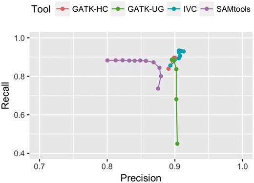
Precision versus Recall of each method for Indel calling at Unknown variant locations as coverage varies from 3× to 50×

3.2.2 Predicting close-by Indels using known variants

Two Indels are considered to be close-by if their left-most ends are located closely to each other. Our analysis of population Indels in human chromosome 1 using variant callset from 1KGP showed that there are 14% of Indels have at least one Indel located within 30 bp on the left or on the right in terms of their left-most positions.

Close-by Indels make it challenging for aligners to get the correct alignments and consequently for variant callers to make the correct calls (Li, 2014). An aligner’s mistake in getting the correct alignment for one read will likely repeats for another read. Therefore, high coverage probably does not help in improving the accuracy of calling close-by Indels. To illustrate this, let’s consider a toy example in which the read GTAATATTGT is aligned to the reference genome GTATTAGTGT:

location 1234567890  1234567890

genome   GT–––ATTAGTGT   GTATTAGTGT 

read    GTAATATT-GT      GTAATATTGT

      correct algn   incorrect algn

The correct alignment yields two Indels at location 2 and 5, while the incorrect one yields two SNPs at location 4 and 7. An aligner likely chooses the incorrect alignment as it has better scores (gaps in Indels are generally penalized seriously by aligners). This can be repeated for all reads thus it makes the alignment based variant callers difficult to detect the correct variants even at high coverage. Our analysis of true positives and false negatives of all four methods confirmed this. They were more likely to detect variants correctly when there were fewer close-by Indels. Counting the number of Indels located within 30 bp on the left or on the right of a variant at coverage 50×, we found that on average, the difference in numbers of close-by Indels between true positives and false negatives for all four methods is approximately 1. Thus, on average, one close-by Indel within a window size of 30 bp could make a difference between one correct call and one incorrect call.

IVC’s ability to detect close-by Indels compared to the other methods is apparent in Table 1. Even at 50×, IVC’s recall rate of Indels was 4–5% higher than that of the other methods. To analyze IVC’s ability to detect these Indels more carefully, we separate them into two main groups, G50 and G100, based on the percentage of known close-by Indels within 30 bp that IVC was informed, 50 and 100%, respectively. Figure 2 shows the numbers of true positives and false negatives of Indels in each of the three groups, for all four methods (AT was eliminated from this experiment due to its too low recall). First, we see that the ratio between true positives and false negatives of UG, HC and ST are, respectively, similar in all groups. This makes sense because these tools are not informed of close-by Indels. Second, the more IVC is informed of close-by Indels, the more likely it is able to detect Indels correctly. In particular, when IVC is totally informed of close-by Indels (G100), the number of true positives and false negatives increased and decreased significantly, respectively, compared to the others. One notice in this experiment is that the numbers of Indels in those groups are non-uniformly distributed. This characteristic of the data caused by our strategy of randomly selecting known/unknown variants for both SNPs and Indels for whole evaluation, not for only this one. Nevertheless, this result could show the advantage of leveraging known information of close-by Indels.

Fig. 2.

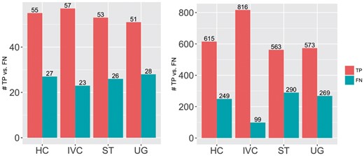
Number of TP and FN of each tool at different fractions of close-by known Indels. Left: 50% of close-by Indels are known, Right: 100% of close-by Indels are known. HC: GATK-HaplotypeCaller, IVC: our tool, ST: SAMtools, UG: GATK-UnifiedGenotyper

3.3 Leveraging known variants to detect variants from Platinum Genomes data

In this section, we compared the ability of detecting variants between IVC and other methods on real data. To accomplish this, we used sequencing reads from human sample NA12878 provided by Illumina Platinum Genomes Project (dataset ERR194147, sequenced at 50×). We used variants from the 1KGP data (Phase 1) (1000 Genomes Project Consortium, 2012) as the known variant profile for IVC. Since this variant dataset does not include the NA12878 individual, the experiment is meant to show how IVC exploits known variants from population to detect variants for a new individual. We also used dbSNP (build 142) (Wheeler et al., 2007) as the known variant profile to investigate more about IVC’s ability of leveraging known information in calling variants. To evaluate accuracy of all methods, we used the Genome-In-A-Bottle variant call set [GIAB (Zook et al., 2014)]. GIAB, which integrated 14 datasets from five sequencing technologies, seven read mappers and three variant callers to help minimize bias toward any method, has been used as gold standard for benchmarking variant calls in many studies (Cornish and Guda, 2015; Li, 2015). In this experiment, GATK UnifiedGenotyper and Atlas2 were eliminated because of their inferior performance on simulated data.

To evaluate the methods, we consider their two main groups of called variants: (i) GIAB-Call, called variants that are in the GIAB; and (ii) GP-Call, called variants that are not in the GIAB but are in 1KGP. The two top diagrams of Figure 3 showed the high sensitivity of IVC compared to HC and ST. We could see that IVC called more unique GIAB-variants than the other methods while sharing with them most of variant calls in this group. This result showed that IVC can reduce the number of false negatives. Further, the number of variants shared between IVC and HC is the highest compared to those between IVC and ST as well as those between HC and ST. This was consistent with the high performance of IVC and HC compared to ST with simulated data.

Fig. 3.

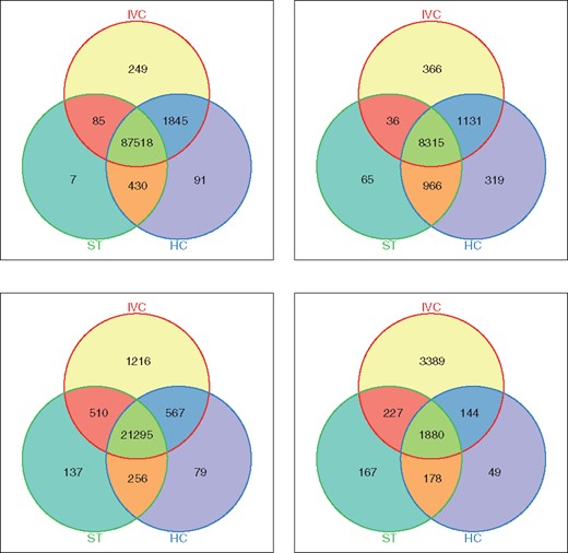
Number of SNPs and Indels called by each method (IVC: our tool, HC: GATK-HaplotypeCaller, ST: SAMtools) from sample NA12878 on Chromosome 1 using Illumina Platinum data. Top: GIAB-Call, variant calls that are in the GIAB dataset (Left: SNPs, Right: Indels). Bottom: GP-Call, variant calls that are not in the GIAB dataset but are in the 1KGP dataset (Left: SNPs, Right: Indels)

The two bottom diagrams of Figure 3 showed another important result, which confirmed the advantage of exploiting known variants by IVC to detect variants. We could see that IVC called much more unique variants that are in 1KGP data, especially Indels, than the other methods. We got ∼9 times more unique GP-Call-SNPs and ∼20 times more unique GP-Call-Indels than the others’. Interestingly, while IVC shared the most number of SNPs with HC, it shared the most number of Indels with ST, compared to the number of sharing variants between all two methods.

For the called variants that are neither in the GIAB dataset nor in the 1KGP data, we found that the agreement between IVC, HC and ST were too low compared to two above groups (∼3100 shared calls for SNP calling and ∼3300 shared calls for Indel calling). In particular, for Indel calling, each method called ∼4000 to 4500 unique variants, which were even more than the common calls. There might be many false positives in such callset of each method, which are worth for further analyses.

Next, we compared all methods using their specificity and sensitivity based on the GIAB variant call set. For SNP calling, IVC got specificity and sensitivity of 99.996 and 99.609%, respectively, while ST got 99.998 and 97.790% and HC got 99.998 and 99.817%, respectively. For Indel calling, IVC got specificity and sensitivity of 99.996 and 90.523%, respectively, while ST got 99.996 and 86.240% and HC got 99.996 and 98.640%, respectively. In this comparison, HC seems to be the best one in term of balance between specificity and sensitivity.

Finally, we tested IVC using dbSNP as known variant profile to investigate more its ability of leveraging existing known variant databases. Because dbSNP does not focus on Indels, we evaluated IVC on SNP calling. Our results showed that IVC with dbSNP got specificity and sensitivity of 99.989 and 98.497%, respectively, while IVC with 1KGP data got 99.996 and 99.609%. Although the performance in both cases are quite similar, it seems that IVC can leverage a bit more from 1KGP data than dbSNP data. This is probably because 1KGP data include allele frequencies, which can help IVC improve detection of variants through its calculation, whereas dbSNP data do not.

3.4 Leveraging known variants to detect exonic Indels

In this section, we compared the ability of detecting exonic Indels of IVC compared to other methods. In terms of known variant sources for IVC, we used ExAC (Lek et al., 2016), a more comprehensive and accurate known variant data compared to 1KGP data, especially for Indels, as described in Section 3.1.1. Although this database is for exonic regions only, we think the evaluation is still important due to the crucial role of the exonic regions in genomic research. In terms of the sequencing read datasets, in addition to the original dataset ERR194147 (50×), we also down-sampled it to 20×, 10× and 5×, respectively, to investigate impact of coverage on performance of each method.

To get a more comprehensive evaluation of the ability of IVC in calling Indels compared to other tools, in addition to GATK HaplotypeCaller and SAMtools, we also considered Scalpel, a more recent Indel caller (Narzisi et al., 2014). Scalpel performed a localized micro-assembly on specific regions of interest to improve detection of variants. Table 3 showed that IVC has competitive to high sensitivity at calling Indels compared to other methods, especially at low coverage. Overall, Scalpel did a good job for calling Indels, especially at high coverage (>10×). However for calling Indels that are in both GIAB and ExAC data (GIAB$\cap$ExAC), IVC was better than Scalpel and other tools, especially at low coverage (<10×). This result again showed the advantage of leveraging known Indels by IVC to detect Indels.

Table 3.

Number of Indels called by each method from sample NA12878 on exonic regions of Chromosome 1 as coverage varies from 5× to 50×

	Tools	5×	10×	20×	50×
GIAB$\cap$ExAC	Scalpel	15	51	59	59
	HaplotypeCaller	57	64	64	64
	SAMtools	52	64	63	63
	IVC	65	66	69	70
GIAB$\cap$NonExAC	Scalpel	10	44	62	71
	HaplotypeCaller	12	13	14	14
	SAMtools	7	8	12	12
	IVC	8	9	10	10

Note: GIAB$\cap$ExAC: variant calls existing in both GIAB and ExAC. GIAB$\cap$Non-ExAC: variant calls existing in GIAB but not in ExAC.

3.5 Runtime analysis

To evaluate computational cost of all methods, we compared their runtime using simulated reads on Chromosome 1 with coverage from 5× to 50×. All experiments were run on a workstation with 2 CPUs Xeon E5-2680 2.70 GHz. We used multi-threaded mode for all tools whenever possible with maximum number of cores (32) (actually all of them had been run in multi-threaded mode with 32 cores except some data preprocessing tasks). We summed up runtime of all steps in whole variant calling pipeline of other methods (aligning the reads, converting SAM files to BAM files, sorting the BAM files, doing post-alignment processing tasks, performing Indel realignment and calling variants). Figure 4 showed that IVC was faster than or at least competitive with the other tools at low to medium coverage and was quite competitive at high coverage.

Fig. 4.

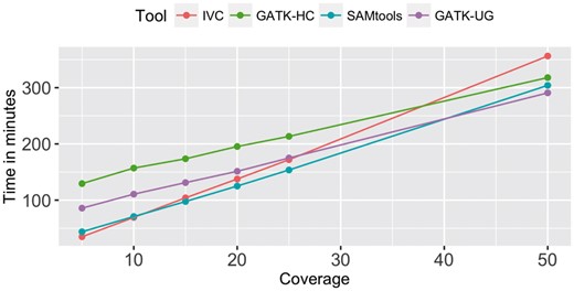
Runtime of all tools with simulated data at various coverages on Chromosome 1

We have also tested our method on simulated whole genome data with all chromosomes using the same above settings. Due to time limit, we selected only GATK HaplotypeCaller for our comparison. Table 4 showed that IVC performed even better than HaplotypeCaller on all chromosomes compared to Chromosome 1. The main reason for that is probably our iterated randomized strategy for searching seeds is able to gain an advantage on high repetitive regions of the other chromosomes.

Table 4.

Runtime (format: hh:mm:ss) of IVC and GATK HaplotypeCaller (HC), including all steps of its pipeline (alignment with BWA, pre/postprocessing, realignment with GATK IndelRealigner, and variant calling with GATK HaplotypeCaller) with simulated data at various coverages on all chromosomes

	5×	10×	20×	30×	50×
BWA-MEM	00:41:16	01:28:27	03:18:31	04:26:46	07:15:00
IndelRealigner	00:55:44	01:22:47	02:33:14	03:51:42	06:21:18
Pre/postprocess	01:27:29	03:42:37	05:43:21	08:33:45	18:07:50
HaplotypeCaller	24:59:05	22:59:45	25:02:22	30:22:27	36:43:14
HC-Total	28:03:34	29:33:36	36:37:28	47:14:40	68:27:22
IVC	04:46:26	09:41:39	20:08:42	30:11:40	53:07:33

4 Discussion

By leveraging known genomic variant information, IVC could significantly improve sensitivity of detecting not only known but also unknown variants, including close-by Indels, one source of hard-to-detect Indels. Compared to other popular methods GATK UnifiedGenotyper, GATK HaplotypeCaller, SAMtools, Atlas2 and Scalpel, IVC had superior sensitivity for calling not only known but also unknown variants, especially close-by Indels that are hard to detect by the others. Its superior sensitivity at low coverage can help researchers design less expensive experiments, especially in case high quality known genomic variants are available.

One important motivation of our work is the number of known genomic variants is rapidly growing. However, variant databases such as the 1000 Genomes Project data or dbSNP are not error-free despite the best efforts. Since our method prefers the know variants if they exist by giving them high prior probabilities in variant profiles, the incorrect known variants can result in false positives. However, our method do not rely on only known variants, it considers the alignment between reads and the reference as well. Those incorrect variants will likely result in the alignments with ambiguities or low quality, which are likely to be eliminated during the alignment process. Consequently, those variants likely do not have high probabilities in the final variant profiles and they are likely not called. This makes our method less suffers from inaccurate known variants.

Currently IVC focuses on detecting SNPs and Indels, long insertions/deletions and other structural variants will be considered in near future by incorporating an assembly-driven module. Our experiments were also performed with haploid data only, detection of higher-ploidy variants have been currently testing. The theoretical framework for higher-ploidy data was the same, with some technical modification to store variants and to update the variant profiles.

In summary, our method is promising in sensitively detecting genomic variants from NGS data, including close-by Indels, which are difficult to be detected by other methods due to low coverage or the hardness of detecting those variants. The current implementation is not optimized but still competitive in performance compared to other popular tools.

Acknowledgements

We would like to acknowledge Ken Chen at The University of Texas MD Anderson Cancer Center for his useful comments on the manuscripts as well as the experiment settings. We also thank Quang Tran at The University of Memphis for his work on part of initial implementation.

Funding

This work was partly supported by National Science Foundation Computing and Communication Foundations NSF CCF-1320297.

Conflict of Interest: none declared.