iCFN: an efficient exact algorithm for multistate protein design

Abstract

Motivation

Multistate protein design addresses real-world challenges, such as multi-specificity design and backbone flexibility, by considering both positive and negative protein states with an ensemble of substates for each. It also presents an enormous challenge to exact algorithms that guarantee the optimal solutions and enable a direct test of mechanistic hypotheses behind models. However, efficient exact algorithms are lacking for multistate protein design.

Results

We have developed an efficient exact algorithm called interconnected cost function networks (iCFN) for multistate protein design. Its generic formulation allows for a wide array of applications such as stability, affinity and specificity designs while addressing concerns such as global flexibility of protein backbones. iCFN treats each substate design as a weighted constraint satisfaction problem (WCSP) modeled through a CFN; and it solves the coupled WCSPs using novel bounds and a depth-first branch-and-bound search over a tree structure of sequences, substates, and conformations. When iCFN is applied to specificity design of a T-cell receptor, a problem of unprecedented size to exact methods, it drastically reduces search space and running time to make the problem tractable. Moreover, iCFN generates experimentally-agreeing receptor designs with improved accuracy compared with state-of-the-art methods, highlights the importance of modeling backbone flexibility in protein design, and reveals molecular mechanisms underlying binding specificity.

Availability and implementation

https://shen-lab.github.io/software/iCFN

Supplementary information

Supplementary data are available at Bioinformatics online.

1 Introduction

Designing proteins of desired structures, properties, or functions would enable unraveling and modulating biological systems and allow for a wide array of applications. Although this important problem remains challenging, progress has been made with computational protein design (CPD), sometimes together with experimental approaches such as directed evolution. CPD introduces an automated and accelerated way to tackle the problem. More importantly, it can rationally generate a tangible number of designs (and their underlying mechanistic hypotheses) which can be experimentally tested to refine our knowledge.

CPD is often formulated as an optimization problem where a utility or objective function summarizing a single or multiple design objectives is optimized over protein sequence space. As protein functions are largely determined by structures and dynamics, evaluating an objective function for any given sequence often involves energy minimization over structures (or conformations). There are two cases of structure-based CPD problems. The first is single-state design that only considers one desired (or ‘positive’) state (e.g. stability of a given, fixed backbone conformation). However, there are two limitations with single-state design: (i) without the explicit consideration of an undesired (or ‘negative’) state, a designed binder may not be foldable or no specificity can be achieved; (ii) without the consideration of multiple positive or negative substates such as conformations, folds, oligomers and on/off-target binding, no multiple sub-objectives, positive or negative, can be accomplished and over-simplified assumptions often have to be made (for instance, a fixed backbone despite that flexible protein structures exist in an ensemble of conformational substates; Frauenfelder et al., 1988; Hartmann et al., 1982). Rather, the second case of CPD—multistate design—removes both limitations by considering both positive and negative states and allowing multiple substates for either state (Harbury et al., 1998). Some ‘multistate’ design studies only remove one limitation thus we emphasize the difference between ‘state’ and ‘substate’ here to remove possible confusions.

Even single-state CPD is extremely challenging. With protein backbones fixed and side chains discretized as rotamers (Dunbrack and Karplus, 1993), the resulting combinatorial optimization problem is nondeterministic polynomial time-hard (NP-hard) (Pierce and Winfree, 2002) thus unlikely has a polynomial-time algorithm. Over the past two decades, three types of algorithms have been developed for single-state design: heuristic, approximation, and exact algorithms, among which only exact algorithms can guarantee the global optimum.

Heuristic algorithms include genetic algorithms (Jones, 1994) and Markov chain Monte Carlo (MCMC) that can generate good-quality feasible solutions efficiently. In particular, MCMC is used in the very popular Rosetta software (Leaver-Fay et al., 2011b) and has led to many successful applications (Ambroggio and Kuhlman, 2006; Bale et al., 2016; Jiang et al., 2008; Kortemme et al., 2004; Kuhlman et al., 2003; Rothlisberger et al., 2008). Approximation algorithms include relaxed integer programing (Kingsford et al., 2005) and loopy belief propagation (Fromer and Yanover, 2008; Yanover and Weiss, 2002) that solve approximate forms of the problem.

Despite progress in heuristic or approximation algorithms for single-state design, there is a critical need for exact algorithms due to two major reasons. First, the guarantee of the global optimum from exact algorithms assures that biophysical models and mechanistic hypotheses underlying the formulation can be isolated from search algorithms and improved based on design success or failure; and the guarantee of a gap-free list of the top sub-optimum directly addresses uncertainty in those biophysical models (such as free energy calculation). Second, the performance gap between exact and heuristic algorithms widens as the size of single-state design grows (Simoncini et al., 2015) and this gap will be even wider for multistate design whose size grows further with the number of substates.

The first and the most known framework of exact algorithms is dead-end elimination (DEE) followed by A* (Gainza et al., 2013; Leach and Lemon, 1998; Lippow et al., 2007; Shen et al., 2013, 2015). DEE is widely used to prune the search space; and A* (Hart et al., 1968) is a tree search algorithm for enumerating a gap-free ordered list in the pruned space. Original DEE criteria (Desmet et al., 1992, 1994) have evolved to more powerful albeit more costly ones (Goldstein, 1994; Gordon and Mayo, 1998; Pierce et al., 2000). Furthermore, the DEE framework has been extended by the Donald group to first consider continuously flexible side-chain rotamers in minDEE (Georgiev et al., 2006) and iMinDEE (Gainza et al., 2012), then locally flexible backbones within voxel boxes (Georgiev and Donald, 2007), and recently both locally flexible backbones and side-chain rotamers in DEEPer (Hallen et al., 2013). Other promising extensions include deriving tighter bounds in BroMAP (Hong et al., 2009) and dynamic A* (Roberts et al., 2015) as well as exploiting the sparseness of protein residue contact maps in AND/OR branch-and-bound search (Zhou et al., 2016).

Recently, a new framework of exact algorithms called cost function network (CFN) has been introduced to re-formulate single-state design as a weighted constraint satisfaction problem (WCSP) (Larrosa, 2002; Schiex et al., 1995) modeled through a CFN and to solve it using depth-first branch-and-bound (DFBB) (Allouche et al., 2012; Traoré et al., 2013). CFN is shown to be significantly faster than other exact methods or solve problems of sizes unprecedented to DEE/A* (Simoncini et al., 2015; Viricel et al., 2018). Various local consistencies have been developed for lower bounding in DFBB (Cooper et al., 2007, 2008; Givry and Zytnicki, 2005; Larrosa and Schiex, 2003, 2004; Nguyen et al., 2017), among which existential directed arc consistency (EDAC) is used the most for its balance between tightness and cost in practice.

However, for multistate protein design with substate ensembles, no exact algorithm exists except an extension of DEE/A*—COMETS (Constrained Optimization of Multi-state Energies by Tree Search) (Hallen and Donald, 2015). Progress has been focused on heuristic or approximation algorithms (Grigoryan et al., 2009; Harbury et al., 1998; Havranek and Harbury, 2003; Leaver-Fay et al., 2011a; Loffler et al., 2017; Negron and Keating, 2013; Sevy et al., 2015). For multistate design, DEE has been extended to type-dependent DEE where only rotamers of the same amino-acid type can prune each other (Yanover et al., 2007). For multistate design where the objective function is a linear combination of substate energies, COMETS incrementally searches for the lowest-scoring sequence with A* by exploiting new lower bounds and generates the top few sequences.

Here we present iCFN (interconnected CFNs), a novel and efficient exact algorithm for generic multistate CPD (with substate ensembles for both positive and negative states). Our optimization formulation is general enough for various design tasks. And our algorithm guarantees a gap-free list of the best sequences and conformations with unprecedented efficiency for practical, large-scale multistate CPD problems. Specifically, we have adopted the formulation of WCSP and the model of CFN for each substate; and represented the coupled WCSPs as iCFNs over a tree of sequences, substates and rotamers (values). Then we have derived novel lower bounds with theoretical proofs and complexity analysis; and we have designed DFBB-based tree search that allows positive and negative designs to inform each other and substates within and across states to prune each other. Finally, we have applied iCFN to designing a T-cell receptor (TCR) to specifically recognize an antigen peptide and avoid another while allowing all molecules’ backbones to be globally flexible. For the resulting multistate CPD problems of unprecedented sizes to exact methods, iCFN drastically improves the efficiency and accuracy compared with state-of-the-art methods and provides new insights into the importance of backbone flexibility in CPD and molecular mechanisms of binding specificity.

2 Materials and methods

2.1 Formulation

We will first introduce and formulate various cases of CPD of increasing computational complexity and biophysical relevance. Bold-faced notations in lower cases indicate vectors.

2.1.1 Single-state design with a single substate

A simple CPD is to find the best sequence s that optimally accommodates a desired (positive) substate as measured in an objective function $f(x)$ of protein structure x. Proteins are often assumed to have fixed backbones and discrete side-chain rotamers r at selected, mutable or flexible residues. So the only non-fixed part of the structure x consists of these side-chain rotamers r. The objective function, often some form of energy functions, is usually assumed to be a sum of constant, singleton, and pairwise terms:

$$f(r)=c+{\displaystyle \sum _{i}E}(i_r)+{\displaystyle \sum _{i<j}E}(i_r,j_s),$$

(1)

where i_r and j_s denote rotamers r and s at residue i and j, respectively. An example of $f(·)$ is the energy $E(·)$ of protein structure x to stabilize a desired, fixed backbone structure potentially for a desired function.

The resulting optimization problem can be formulated as

$$s^{\ast }=arg\underset{s\in \mathcal{S}}{\min }\underset{r\in \mathcal{R}(s)}{\min }f(r),$$

(2)

where the set $\mathcal{S}$⁠, capturing the sequence design space, is the Cartesian product of the sets of amino-acid types allowed over all residues; and $\mathcal{R}(·)$⁠, capturing the rotamer library, is the Cartesian product of the rotamer sets over all mutable or flexible residues of a sequence.

2.1.2 Single-state design with substate ensembles

This slightly more complex case also considers just positive design (or state) but considers an ensemble of positive substates rather than one. Such treatment leads to more accurate biophysical models and more design capabilities. For instance, it allows for treating a protein backbone flexible when these substates correspond to backbone conformers; and it allows for designing binding profiles when these substates correspond to various ligand-bound states. We give the formulation as

$$s^{\ast }=arg\underset{s\in \mathcal{S}}{\min }\underset{p\in \mathcal{P}}{\min }\underset{r\in {\mathcal{R}}_p(s)}{\min }{f}_p(r),$$

(3)

where $\mathcal{P}$ is the set of positive substates and $f_p(·)$ is the objective function for the pth positive substate. Minimizing over $\mathcal{P}$ substate objective functions $f_p(·)$ maintains an ‘OR’ relationship among them for the overall (positive) objective. For instance, in the case of $f_p(·)$ being energies $E_p(·)$⁠, it ensures choosing the ground substate with its sequence and conformation being optimized simultaneously. One can also maximize over $\mathcal{P}$⁠.

2.1.3 Multistate design with a single substate per state

When compared with the two previous cases with positive state only, this case considers both positive and negative states each represented by a single substate. In other words, it is to find the best sequence that specifically accommodates a desired positive substate rather than an undesired negative substate. The objective function here can be the gap between the two substate objective functions $f^{\text{+}}(·)$ and $f^{\text{-}}(·)$⁠. The formulation is given as

$$s^{\ast }=arg\underset{s\in \mathcal{S}}{\min }\left(\underset{r\in {\mathcal{R}}^{\text{+}}(s)}{\min }{f}^{\text{+}}(r)-\underset{r\in {\mathcal{R}}^{\text{-}}(s)}{\min }{f}^{\text{-}}(r)\right),$$

(4)

where superscripts ‘+’ and ‘−’ indicate positive and negative quantities, respectively. For instance, this formulation allows for binding affinity design when positive and negative substate objective functions are energies of a protein in one bound and one unbound state, respectively. It also allows for binding specificity design when these substate objective functions are binding energies to one target and one off-target, respectively.

2.1.4 Multistate design with substate ensembles

The most generic formulation, for which our exact algorithm will solve, considers both positive and negative states explicitly and considers an ensemble of substates for either state. The formulation can be written as

$$s^{\ast }=arg\underset{s\in \mathcal{S}}{\min }\left(\underset{p\in \mathcal{P}}{\min }\underset{r\in {\mathcal{R}}_p^{\text{+}}(s)}{\min }{f}_p^{\text{+}}(r)-\underset{q\in \mathcal{Q}}{\min }\underset{r\in {\mathcal{R}}_q^{\text{-}}(s)}{\min }{f}_q^{\text{-}}(r)\right),$$

(5)

where $\mathcal{P}$ and $\mathcal{Q}$ denote the positive and the negative substate ensemble with p and q being the positive and negative substate index, respectively. Moreover, constraints on substate objective functions can be introduced and addressed (e.g. those linear ones in our TCR design).

This generic formulation includes all aforementioned formulations as special cases. It helps improve the accuracy of biophysical models and strengthen the capability to design for multiple desired substates over multiple undesired ones. For instance, one can design a tight binder that can fold using protein-complex and binder alone as positive and negative states in conformational ensembles, respectively, as our XRCC1 design does in Section 3.1. One can also design a protein that specifically binds to a target ‘ensemble’ rather than an off-target one with $f_p(·)$ and $f_q(·)$ being energies for the pth target and qth off-target, respectively, as our TCR design does in Section 3.2. The $\min$ operator over all positive substates can be replaced by max for multi-specificity and solved similarly.

2.2 iCFN for multistate design with substate ensembles

With the generic formulation given, we proceed to introduce our exact algorithms based on CFNs. CFN is the state-of-the-art approach to single-state protein design with a single substate (Allouche et al., 2012; Traoré et al., 2013). We extend CFN for multistate design with substate ensembles. We first design a tree structure of sequences, substates, and rotamers and a tree-search algorithm using CFN as a corner stone, which leads to a reduced version of the ultimate iCFN. Here CFN is used to solve each substate energy minimization problem for any given sequence, a problem also known as side-chain packing (SCP). We further improve the reduced version to iCFN by deriving novel bounding schemes across CFNs.

A high-level schematic illustration of iCFN is shown in Figure 1. For either positive or negative state, iCFN first reads data (singleton and pairwise energy values) and prunes the search space using type-dependent DEE within and across substates sequentially. Individual substate designs are reformulated as WCSPs and modeled with iCFNs over a tree representation of the search space. Using a DFBB approach, iCFN then searches over sequence space with newly proposed and proven lower bounds to prune partially or fully defined sequences and searches over substate-rotamer space for un-pruned, fully defined sequences (i.e. SCP). After the global optimum is found, it will redo DEE pruning and DFBB search with updated bounds and relaxed energy thresholds for an ensemble of the best sequences in an ensemble of the best positive and negative conformations.

Fig. 1.

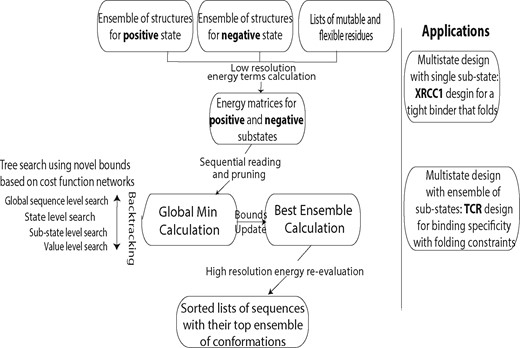
Schematic illustration of the study: algorithm design and application

Next we will explain these steps in more details. In the interest of space, we place all proofs and pseudocodes in the Supplementary Material.

2.2.1 Sequential reading and pruning of rotamers

iCFN first sequentially reads data and incrementally prunes rotamers for either state. When reading each substate, it prunes rotamers within the substate using type-dependent DEE—Goldstein and single split DEE for all substates as well as single pair and single double DEE just for positive substates. It then prunes rotamers for substates read so far using our extended, across-substate type-dependent DEE. This approach drastically reduces peak memory usage to store substate rotamers. We provide its flowchart and pseudocode in Supplementary Figure S1 and Algorithm 1, respectively.

We extend within-substate type-dependent DEE (Yanover et al., 2007) to across-substate type-dependent DEE as follows: 

Theorem 1.

Rotamer i_a of position i in Substate 1, provably pruned by rotamer i_b of the same position in Substate 2, is not part of the optimal solution if both substates are of the same state, both rotamers are of the same amino-acid type, and the following criterion holds:

$$\begin{array}{c}{L}_1(i_a)=c_1+E_1(i_a)+{\displaystyle \sum _{j,j\ne i}\underset{s_1}{\min }}(E_1(j_{s_1})+E_1(i_a,j_{s_1}))\\ +{\displaystyle \sum _{j>k,k\ne i,j\ne i}\underset{s_1,u_1}{\min }}{E}_1(j_{s_1},k_{u_1})>U_2(i_b)=c_2+E_2(i_b)\\ +{\displaystyle \sum _{j,j\ne i}\underset{s_2}{\max }}(E_2(j_{s_2})+E_2(i_b,j_{s_2}))\\ +{\displaystyle \sum _{j>k,k\ne i,j\ne i}\underset{s_2,u_2}{\max }}{E}_2(j_{s_2},k_{u_2})\end{array}$$

(6)

An extension for the top δ-kcal/mol ensemble is that rotamer i_b of Substate 2 prunes rotamer i_a of Substate 1 if $L_1(i_a)>U_2(i_b)+\delta$⁠. In some applications especially for the optimal ensemble, these across-substate DEEs can increase computational cost more than they add pruning power and thus can be disregarded in iCFN as we later do for TCR design.

2.2.2 Global sequence-level search

The second stage of iCFN performs DFBB search over the sequence space that is represented in a hierarchical tree structure together with states, substates, and conformations. The overall search strategy is illustrated in Figure 2. Beginning with a completely undefined sequence indicated by all ‘X’, it splits the current sequence space (parent node) into two subspaces (child nodes), based on the first amino acid being valine (V) or not. It then evaluates the lower bound on the right child corresponding to a partially defined sequence and determines whether to prune its entire subtree or to split it again. The so-called binary branching repeats until reaching a sequence-level leaf node (i.e. a fully defined sequence) whose lower bound is evaluated for pruning. If the sequence is not pruned, state, substate, and rotamer-level search follows with similar DFBB (next subsections). Then iCFN calculates the sequence’s specificity score and updates the upper bound for optimal specificity if the score is lower than the best specificity so far.

Fig. 2.

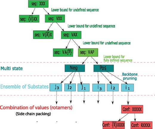
Schematic illustration of global sequence search

Two types of lower bounds with proofs (Supplementary Material) and complexity analysis are developed for iCFN to prune sub-trees of sequences (including their associated substates and rotamers) when the search reaches a sequence-level leaf node (i.e. a fully defined sequence) or otherwise. They are not included in reduced iCFN to assess their sole contribution to numerical efficiency.

The first lower bound is generically applicable to all sequences, fully defined or not. Details and proofs can be found in Supplementary Material. 

Theorem 2.

For any sequence space S, a lower bound of the objective function for multistate protein design with substate ensembles [Formulation in Equation (5)] is given by (× denotes Cartesian product):

(7)

$$\begin{array}{l}\Delta c_{kl}=c_k^{\text{+}}-c_l^{\text{-}},\\ \Delta E_{kl}(i_{r,r\prime })=E_k^{\text{+}}(i_r)-E_l^{\text{-}}(i_{r\prime }),\\ \Delta E_{kl}(i_{r,r\prime },j_{s,s\prime })=E_k^{\text{+}}(i_r,j_s)-E_l^{\text{-}}(i_{r\prime },j_{s\prime }),\end{array}$$

(8)

i.e. differences in constant, singleton and pairwise energies between a positive substate k and a negative substate l.

We also give the time complexity of the lower bound as follows. By using a lookup table of size $O(n^{2}a)$ that contains minimal/maximal energy between all position pairs for each positive/negative substate, we accelerate this lower bound calculation by O(r). 

Theorem 3.

The lower bound in Theorem 2 can be computed in $O({(nRa)}^{2}r)$⁠, where n is the number of positions, R the average number of rotamers per position, a the average number of substates per state, and r the average number of rotamers per amino acid.

In practice, we only use the first lower bound for partially defined sequences and have derived a tighter one for fully defined sequences: 

Theorem 4.

For any fully defined sequence s, a lower bound can be given by

$$\underset{k\in \mathcal{P}}{\min }{L}_k^{\text{+}}(s)-\underset{l\in \mathcal{Q}}{\min }{U}_l^{\text{-}}(s)$$

(9)

in which $L_k^{\text{+}}(s)$ is the lower bound on all rotamers for sequence s and kth substate in positive design and $U_l^{\text{-}}(s)$ is the upper bound on all rotamers for sequence s and lth substate in negative design.

We use EDAC to calculate the lower bound and limited discrepancy search (LDS) to calculate the upper bound for a fully defined sequence.

Last, we can allow at most M mutations among all mutable positions using LDS again (pseudocode included as part of Algorithm 3 in the Supplementary Material).

2.2.3 State and substate-level search

Once a fully defined sequence s is reached and cannot be pruned, it splits into child nodes of positive and negative states and follows positive substates then negative ones. iCFN repeats DFBB in the rotamer space for SCP in each substate. We use the following bounding criteria to prune substates.

• Within the same state: Substate k prunes l if they are in the same state (positive/negative) and $U_k^{·}(s)<L_l^{·}(s)-\delta$ where the superscript $·$ stands for either $\text{+}$ or $\text{-}$⁠. We again use EDAC and LDS for $L_l^{·}(s)$ and $U_k^{·}(s)$⁠, respectively.

• Across the two states: For a negative substate q, all the subsequent negative substates will be skipped if no rotamers both pass the within-state pruning and satisfy $\min \{f^{\text{+}}(s)\}-f_q^{\text{-}}(·)<S_{\text{best}}+\varepsilon$⁠, where $\min \{f^{\text{+}}(s)\}$ denotes the optimal value among all positive substate functions for the sequence s and $S_{\text{best}}$ is the lowest (best) specificity score of the best sequence so far. If q = 1 (the first negative substate), the sequence s is also pruned.

There might be more substate constraints in practice. For instance, our TCR design formulation has a stability condition for positive substates: $L_p^{\text{+}}(s)>\min \{f^{\text{+}}(\text{WT})\}+\tau$⁠. Therefore, a positive substate p is pruned if its stability lower bound is worse than wild type by more than τ. Other user-defined constraints on substates can further speed up the search.

2.2.4 Value-level (rotamer) search (side-chain packing)

Once reaching a substate that is not pruned, iCFN again uses binary branching to iteratively split during search the conformational space into a chosen rotamer and all the rest. For pruning conformational subtrees, the search again uses EDAC as lower bounds and LDS as upper bounds in each SCP. After a leaf node of the tree (a fully defined conformation for a fully defined sequence) is visited and cannot be pruned, it either becomes the best solution so far or enters the δ-ensemble for the corresponding sequence in the substate. The ensemble size for each sequence in each substate can be limited to K where the K choices can be the first or the best (implemented with a max-heap data structure).

2.2.5 Backtracking

When a sequence- or rotamer-level node is pruned with its subtree, our tree search backtracks to its parent node, re-orders variables (positions) and values (amino acids or rotamers) in the tree (see ordering in the next subsection), and repeats the DFBB process.

2.2.6 Ordering

The ordering of positions, amino acid types and rotamers in the search tree also has an impact on the pruning efficiency. We use several ordering heuristics, originally developed for constraint satisfactory problems (CSPs) and later extended for weighted CSPs, to boost the speed of iCFN without compromising its guarantee of the global minimum or the gap-free top list.

For variable (position) ordering, the state of the art is the increasing order by the number of amino acids or rotamers over the median of pre-calculated energy terms for global sequence search or SCP, respectively. The principle is to visit nodes of higher energies earlier to prune their child nodes more likely and visit nodes of fewer combinations to prune more or bigger subtrees. We improve the efficiency for iCFN by using the median of singleton terms only. The rationale is that singleton terms (e.g. interactions between side chains and backbones) often dominate over pairwise terms in SCP problems (Desmet et al., 2002; Eisenmenger et al., 1993). Note that this treatment does not affect the accuracy of iCFN. In practice it may lead to slightly increased number of nodes expanded or leaves visited but still saves running time with much less time spent on each node for bound estimation. More results on this treatment can be found in Supplementary Tables S1 and S2.

For amino acid ordering per position, the wild type is by default the first and the rest is ordered by increasing singleton energy values. And rotamer ordering for each amino acid type is again by the increasing order of singleton energy values. These two orderings are following the principle of increasing the chance to find a good feasible solution early.

2.3 Test on TCR design

We will now introduce the design problem to test our algorithms, with formulation specifics and implementation details.

2.3.1 Background

TCRs recognize peptide antigens presented by major histocompatibility complex (MHC) and play a critical role in the immune response. Therefore, TCRs have been actively pursued for cancer immunotherapy. For instance, the first TCRs developed for melanoma are DMF4 and DMF5 which recognize two structurally distinct peptide epitopes of MART-1 (melanoma antigen recognized by T cells 1) bound to MHC Class I protein Human Leukocyte Antigen (HLA)-A*0201 (HLA-A2). Regulation of redesigned TCR with high affinity and specificity toward target peptide-MHC (pMHC) has been a major task to develop effective TCR-based immunotherapies. Whereas improving binding affinity has represented major efforts so far because of TCRs’ relatively weak binding to pMHC, such improvements often come at a cost of binding specificity to target peptides and thus bring the risk of off-target effects (for instance, strong affinity to MHC regardless of peptide antigens). In addition, evidence shows that TCR affinity above a certain threshold would cause T-cell responsiveness to attenuate. In total, there is a pressing need for the rational design of TCRs of carefully tailored affinity and specificity profiles.

We used the example of TCR DMF5 (Pierce et al., 2014) to design optimal binding specificity while constraining the target-complex folding stability. The target, AAG peptide, is MART-1 non-americ epitope (AAGIGILTV) and the off-target, ELA peptide, is MART-1 decameric epitope (ELAGIGILTV). We modeled global backbone flexibility of bound DMF5, peptides and MHC with a conformational ensemble sampled by molecular dynamics (MDs) simulations.

2.3.2 Biophysical model

Each conformation of TCR-pMHC in the ensemble was treated as a substate. A hierarchy of energy models is used. (i) During the tree search, folding energy (stability) of TCR-pMHC was used as the substate function. Energy terms included Coulomb electrostatics, van der Waals and internal energies as calculated in a CHARMM22 force field as well as nonpolar contributions of hydration energy based on solvent-accessible surface area. (ii) After iCFN generates the top sequence-conformation ensemble, binding energy difference between the target and the off-target (specificity) was used as the overall objective. Folding energies were re-evaluated with a higher-resolution energy model where implicit-solvent Poisson-Boltzmann electrostatics replaces Coulombic electrostatics (Shen, 2013; Shen et al., 2015). Binding energy for the lowest folding-energy conformation was reported for each sequence in each substate.

2.3.3 Substate ensembles

Both peptides were previously crystallized in complex with MHC HLA-A2 or TCR DMF5 and available with PDB accession codes 3QDJ or 3QDG. Both structures were first minimized using a molecular modeling software CHARMM in a CHARMM22 force field with missing residues and atoms added. They were then solvated using VMD with explicit water molecules of 10 Å padding thickness from the molecular boundary and ionized to reach neutral charge and a concentration of 0.145 M. Either system was minimized for 5000 steps and a 10-ns MD simulation was performed using a computer program NAMD2. Starting from the beginning of MD simulations, snapshots were retained every nano-second. In total, there are 11 positive and 11 negative substates.

2.3.4 Computational mutagenesis

We chose four positions as in an earlier study (Pierce et al., 2014): residues 26 and 28 on the α chain of DMF5 and residues 98 and 100 on the β chain. Each mutable position is allowed for 26 amino-acid types (some amino acids with multiple protonation states are each counted more than once). Since folding energy was first used, specificity cutoff ɛ and positive-substate stability cutoff τ were set loose at 1000 kcal/mol while ensemble cut-off δ per sequence at 2 kcal/mol. iCFN searched for the best K = 1000 conformations for each sequence. To reduce conformational representatives for higher-resolution energy evaluation while maintaining diversity, top conformations of each sequence in each substate were geometrically grouped (Lippow et al., 2007) and only the representatives were evaluated for higher-resolution folding and binding energies.

3 Results and discussion

3.1 Numerical comparison to COMETS

We first compare iCFN to the only alternative exact method for multistate protein design, COMETS (Hallen and Donald, 2015), released in OSPREY V2.2 (Gainza et al., 2013). COMETS uses the weighted sum of substate energies as its objective function, which differs from our formulation in Equation (5). So we resort to compare the methods using the same objective function (without constraints), energy calculations and rotamers (without continuous ones) as in OSPREY, which leads to multistate design with a single substate per state as in Equation (4). Specifically, the task is to minimize the binding energy of a protein complex (XRCC1 N-term domain and DNA polymerase beta; PDB code: 3K75) as the difference between the bound (or positive) and the unbound (or negative) state (Hallen and Donald, 2015).

Out of five positions in XRCC1 (residues 391, 409, 411, 422 and 424), we incrementally choose the first N_mut to be mutable; and for each choice of mutable residues, we set all the N_flex residues within $d=$ 3 or 6 Å to be flexible, and increasingly demand the top affinity sequence ensemble (ɛ = 0.5, 1.0 and 1.5 kcal/mol while δ stays at 2 kcal/mol).

From Table 1 we conclude that our algorithms outperform COMETS in both memory usage and CPU time, which enables large designs in practice. Whereas COMETS couldn’t handle designs of more than two mutable positions under a 20-Gb memory limit, reduced iCFN and iCFN can design for all five positions operating below 80-Mb memory. For the single and double designs where all algorithms produced results, reduced iCFN and iCFN are faster than COMETS by one to two orders of magnitude.

Table 1.

Search space statistics and running time (in seconds) comparison between COMETS, reduced iCFN, and iCFN over a series of incrementally larger multi-state XRCC1 design problems with a single substate for either positive or negative state

					ɛ = 0.5 kcal/mol			1 kcal/mol			1.5 kcal/mol
$N_{\text{mut}}$	d(Å)	$N_{\text{flex}}$	Pre-DEE Size	Post-DEE Size (Ensemble)	COMETS	Reduced iCFN	iCFN	COMETS	Reduced iCFN	iCFN	COMETS	Reduced iCFN	iCFN
1	3	9	2.88e17	2.04e8	4.03	0.02	0.02	4.27	0.03	0.3	4.37	0.03	0.03
1	6	16	5.24e30	2.75e19	6.84	0.16	0.12	6.97	0.17	0.12	7.72	0.19	0.13
2	3	10	1.00e22	1.73e12	6.85	0.28	0.15	8.36	0.28	0.16	9.29	0.28	0.16
2	6	19	5.88e37	1.58e25	19.46	2.63	1.41	29.07	2.67	1.44	29.27	2.79	1.47
3	3	11	7.94e27	8.31e18	M	12.64	6.15	M	12.67	6.51	M	12.65	6.54
3	6	20	1.81e43	1.44e30	M	62.17	32.9	M	62.22	33.26	M	62.31	33.47
4	3	14	6.54e36	8.31e26	M	493.26	268.28	M	493.31	268.3	M	493.95	268.41
4	6	26	7.94e56	4.36e38	M	2060	1458	M	2156	1493	M	2161	1498
5	3	15	3.54e42	2.34e30	M	9810	5570	M	9943	6005	M	10 046	6040
5	6	26	1.65e61	1.58e42	M	49 373	37 198	M	49 978	37 223	M	50 405	39 553

Note: ‘M’ indicates an out-of-memory error under a 20-Gb limit.

Theoretical reasons underlie the better performance of our algorithms. On the memory demand, the space complexity of our DFBB is O(N) where N is the number of mutable and flexible positions whereas that of A* used in COMETS is $O(e^N)$⁠. On the computational speed, CFN-based DFBB enjoys stronger lower and upper bounds. Specifically, (i) DFBB uses lower bounds such as EDAC which proved more powerful than partial forward checking-directed arc consistency (PFC-DAC) used in DEE/A* (Allouche et al., 2014). In particular, even when it could not prune the whole subtree for a given position, EDAC can still reduce the subtree size by pruning rotamers of the remaining positions. (ii) For larger problems, DFBB often reaches good-quality solutions much faster than A*, which provides tighter upper bounds earlier.

3.2 TCR design: efficiency

We now apply iCFN to TCR design described in Methods. As shown later, these multistate designs with substate ensembles and dense rotamer libraries are even larger than those with single substates seen in XRCC1 designs. Therefore, we could not apply COMETS under our cluster’s memory and CPU-time limits (50 Gb and 7 core days). Instead, we compare exhaustive search, reduced iCFN (separate CFNs for individual substates), and iCFN to evaluate the benefit of treating CFNs jointly for powerful substate pruning during search.

3.2.1 Reduction in the sequence and conformer spaces

We compare the effective size of the search space after DEE pruning among exhaustive search, reduced iCFN, and iCFN, using the following metrics: (i) the number of fully defined sequences searched, which is the same for exhaustive search and reduced iCFN but much lower for iCFN; and (ii) the number of conformers searched, which, for reduced iCFN and iCFN, include not only leaves (fully defined conformations) visited but also nodes (partially defined conformations) expanded at the rotamer level of SCP for those sequences searched. These results are summarized in Table 2 for the global optimum-specificity sequence and Table 3 for the top ɛ-kcal/mol ensemble (⁠$\varepsilon =3$⁠) of sequences.

Table 2.

Comparing search space statistics and running time between reduced iCFN and iCFN for global optimum in multi-state TCR design with substate ensembles

			Reduced iCFN				iCFN
Position(s)	Pre-DEE Size	Post-DEE Size	Nodes Expanded	Leaves Visited	Sequences	Time (s)	Nodes Expanded	Leaves Visited	Sequences	Time (s)
26	e61	e27	2.45e3	1.41e2	26	1.46	8.55e2	36	3	0.56
28	e66	e49	3.75e4	1.26e3	26	24.5	4.12e3	114	4	6.29
98	e58	e42	2.51e4	8.16e2	25	9.98	2.11e3	88	8	3.38
100	e84	e56	4.92e4	1.75e3	26	19.85	3.78e3	101	3	4.44
26, 28	e87	e62	1.46e6	3.75e4	676	1335.95	5.99e4	791	40	228
26, 98	e119	e68	1.74e6	3.88e4	650	809.18	9.85e3	231	14	182.10
26, 100	e142	e82	4.08e6	1.02e5	676	1510.03	1.01e4	234	5	303.64
28, 98	e126	e92	5.20e6	9.34e4	650	3707.04	3.04e5	4568	106	745.84
28, 100	e141	e104	9.78e6	1.80e5	676	5603.60	2.00e4	349	8	796.96
98, 100	e112	e88	6.03e6	9.34e4	650	4384.48	3.39e4	633	19	526.97
26, 28, 98	e146	e106	1.68e8	2.66e6	16 900	133 672	7.09e5	8171	180	16879
26, 28, 100	e161	e122	2.94e8	5.11e6	17 576	205 865	4.41e4	652	14	22 941
26, 98, 100	e169	e117	3.28e8	4.32e6	16 900	202 001	1.88e5	2425	55	23 430
28, 98, 100	e168	e134	5.86e8	7.35e6	16 900	496 051	7.45e5	8284	103	46 685

Table 3.

Comparing search space statistics and running time between reduced iCFN and iCFN for the top sequence ensemble in multi-state TCR design with a substate ensemble per state

			Reduced iCFN				iCFN
Position	Pre-DEE Size	Post-DEE Size	Nodes expanded	Leaves visited	Sequences	Time (s)	Nodes expanded	Leaves visited	Sequences	Time (s)
26	e61	e54	6.35e4	6.20e4	26	66.69	6.14e3	6.00e3	10	21.86
28	e66	e61	5.92e4	5.70e4	26	114.22	4.09e3	4.00e3	2	23.55
98	e58	e55	5.15e4	5.00e4	25	103.29	4.16e4	4.00e4	20	43.35
100	e84	e77	7.43e4	7.11e4	26	154.51	5.19e3	5.00e3	2	23.74
26, 28	e87	e82	1.70e6	1.62e6	676	7454.93	9.44e3	9.00e3	4	1063.89
26, 98	e119	e111	1.82e6	1.73e6	650	15 449.04	2.51e5	2.38e5	108	3872.32
26, 100	e142	e132	1.89e6	1.75e6	676	19 780.68	2.62e4	2.40e4	10	2226.52
28, 98	e126	e119	1.45e6	1.37e6	650	23 378.51	3.13e4	3.00e4	13	2810.31
28, 100	e141	e132	1.77e6	1.60e6	676	24 631.34	4.22e3	4.00e3	2	2359.10
98, 100	e112	e106	1.60e6	1.51e6	650	17 303.91	3.98e4	3.80e4	19	2056.47
26, 28, 98	e146	e141	—	—	16 900	—	5.86e4	5.50e4	27	105 343
26, 28, 100	e161	e154	—	—	17 576	—	1.48e4	1.40e4	6	99 012
26, 98, 100	e169	e161	—	—	16 900	—	6.76e4	6.00e4	27	185 886
28, 98, 100	e168	e162	—	—	16 900	—	3.73e4	3.40e4	12	158 995

Note: ‘—’ indicates an out-of-time error under a 7-day limit. Note that the ensemble versions are run after corresponding global optima are derived to reach tight sequence-level specificity bounds and their statistics do not include those in the global optimum stage reported in Table 2.

As seen in both tables, the TCR design problems feature sizes unprecedented to exact protein-design methods even after type-dependent DEE: up to ${10}^{56}$ (⁠${10}^{82}$⁠), ${10}^{104}$ (⁠${10}^{132}$⁠) and ${10}^{134}$ (⁠${10}^{162}$⁠) for global optimum (ensemble) single, double and triple designs, respectively.

Reduced iCFN drastically shrinks the conformational space for search. For the global optimum, it only evaluates up to the order of ${10}^2\text{,\hspace{0.17em}}{10}^5$ and ${10}^6$ fully defined conformations and up to the order of ${10}^4\text{,\hspace{0.17em}}{10}^6$ and ${10}^8$ partially defined conformations en route for single, double, and triple designs, respectively. This space-reduction power does not weaken significantly with the increase of the space size as type-dependent DEE does. For the top ensemble, it still only evaluates to the order of ${10}^4$ and ${10}^6$ fully-defined conformations or partially defined conformations en route for single and double designs, respectively.

iCFN shows even more space-reduction power compared with reduced iCFN because, unlike the latter, it reduces the sequence space (and associating substrees) besides the conformational space. In fact, iCFN visits on average 6.7 (7.4), 58.8 (110.8) and 455.1 (1397.2) times less sequences for the best single (ensemble of) sequence(s) in single, double, and triple designs, respectively. Therefore, iCFN for global optimum impressively only evaluates to the order of ${10}^2\text{,\hspace{0.17em}}{10}^3$ and ${10}^3$ fully defined conformations and ${10}^3\text{,\hspace{0.17em}}{10}^5$ and ${10}^5$ partially defined conformations en route, which translates to 9.2, 214.7 and 2358.6 times more space reduction on average compared with reduced iCFN, for single, double and triple designs, respectively. For the top ensemble, iCFN has similar space-reduction improvement compared with reduced iCFN and visits only up to ${10}^5$ conformations, fully or partially defined, to solve triple designs that could not be handled by reduced iCFN within 7 CPU days.

3.2.2 Acceleration in running time

Since search space reduction can come at a cost of relatively expensive bound calculations, we proceed to compare running time in Table 2 for the global-optimum sequence and Table 3 for the top sequence ensemble. The design jobs (especially for the top ensemble) are daunting for an exhaustive search or even COMETS. So we only compare between reduced iCFN and iCFN to examine the algorithmic benefits of interconnections among substate CFNs. The pre-search step of sequential reading and pruning of rotamers is the same between both and excluded in running time reported.

iCFN drastically accelerates conformational search even compared with reduced iCFN and the acceleration is observed to improve with the increase of the problem complexity. Specifically, iCFN runs 3.4, 5.9 and 9.0 times faster than reduced iCFN does for global optimum in an average single, double and triple design, respectively. For the top ensemble, iCFN runs 4.2 and 7.8 times faster than reduced iCFN does in an average single and double design, respectively; and it solves triple designs within 1–2 CPU days whereas reduced iCFN could not within 1 CPU week. The results show that the benefit of pruning power clearly outweighs the burden of bound calculations.

3.2.3 Performance improvement versus problem complexity

In Figure 3 we summarize how much the power of sequence bounding among CFNs grows with the increase of the problem complexity. iCFN manifests its power in reducing sequence space and running time even more with the increase of problem complexity when more positions are mutated or more top solutions are desired. Additional algorithmic contributions to performance improvement are discussed in the Supplementary Material.

Fig. 3.

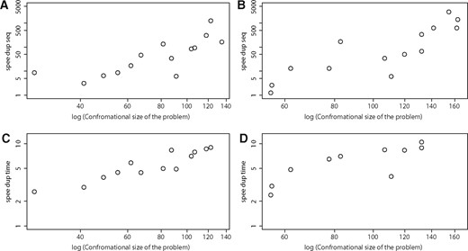
When compared with reduced iCFN, the speedup of iCFN in the number of sequences explored for (A) the global optimum and (B) the best ensemble as well as that in running time for (C) the global optimum and (D) the best ensemble.

3.3 TCR design: accuracy

3.3.1 Comparison to experimental results and Rosetta

We list all TCR designs predicted to be AAG-specific, using an ensemble of backbone structures, in the Supplementary Table S3. When comparing these results to experimental results reported earlier (Pierce et al., 2014), we found that iCFN correctly predicted almost all known AAG-specific TCRs. Specifically, seven AAG-specific mutants involving four residues were previously reported, including α chain D26W, G28L, G28I, G28Y and G28N as well as β chain F100Y and F100W (βL98W is excluded for its specificity being below experimental error bar). iCFN correctly predicted 6 of the 7 (missing G28N) and produced a false positive (FP) D26Y. In contrast, when Pierce et al. used Rosetta V2.3 (Leaver-Fay et al., 2011b) for specificity design, they only found 3 (all at residue 28 and missing G28N as well).

To assess iCFN’s conformational search and energy models, we also compare computed and measured relative binding affinities (⁠$\Delta \Delta G$⁠) as well as binding specificities (⁠$\Delta \Delta \Delta G$⁠) for the six correct designs (G28N not included) and D26Y. For $\Delta \Delta G$⁠, iCFN achieved a Pearson correlation coefficient of 0.52, which is between that of Rosetta with interface backbone minimization (0.39) and Rosetta without (0.62) (Pierce et al., 2014). iCFN’s $\Delta \Delta G$ values over-estimated weak binding affinities for ELA, possibly due to its lenient DEE-pruning and constraints for negative substates. Using $\Delta \Delta \Delta G<0$ calculated to predict specificity, we find in Table 4 that Rosetta led to one FP and two false negatives (FN) and Rosetta Min did three FNs (Pierce et al., 2014) whereas iCFN found the most true positives (TP) with only one FP and no FN.

Table 4.

AAG-specificity predictions by Rosetta, Rosetta Min and iCFN

Method	TP	FP	FN
Rosetta	G28I, G28L, G28Y, F100W	D26Y	D26W, F100Y
Rosetta Min	G28I, G28L, G28Y	N/A	D26W, F100W, F100Y
iCFN	D26W, G28I, G28L, G28Y,	D26Y	N/A
	F100W, F100Y

3.3.2 The impact of substate ensemble and backbone flexibility

We also perform a multistate design with a single substate for either state (i.e. a fixed backbone conformation) and list TCR designs predicted to be AAG-specific in Supplementary Table S4. Whereas a flexible-backbone treatment correctly predicted 6 of 7 AAG-specific mutants, a fixed-backbone treatment only did for 3 (G28L, F100W and F100Y). In fact, for the flexible-backbone treatment, various backbone conformations were adopted in iCFN for various successful designs in the AAG- or ELA-bound complex (see Supplementary Table S5). These results echo the biophysical concept of protein conformational substates and highlight the importance of backbone flexibility to multistate protein design for more diverse solutions and higher success rates.

3.3.3 Characterization of the design space

Beyond individual predictions, iCFN effectively produced energetic landscapes in the design space by generating the top sequences and conformation ensembles. Although conformational flexibility is limited, it predicted that position 98 on the α chain, having much less sequence solutions and worse binding affinities, is much less ‘designable’ for AAG-specificity compared to the other three positions, which agrees with previous experimental observations (Pierce et al., 2014). Other potentially promising designs for AAG-specificity can be found in Supplementary Table S3.

3.3.4 Molecular mechanisms for AAG-binding specificity

Our results correctly predicted that introducing bulkier hydrophobic residues properly to position 26/28/100 could improve binding specificity. Moreover, consistent with experimental results, they predicted various patterns for AAG-specificity including (i) strengthening AAG-binding but weakening ELA-binding (G28I); (ii) strengthening both binding but more to AAG (D26W); and (iii) weakening both binding but less to AAG (G28Y and F100W/Y). They also correctly predicted G28L to have weakened binding to ELA but incorrectly predicted its improved binding to AAG.

Taking G28I as an example, we examine the mutant’s energetic and structural consequences in details. Our results show that G28I achieves binding specificity by exploiting the peptide sequence difference, namely the N-terminus being alanine in AAG but glutamate in ELA. Specifically, a bulkier I28 would strengthen interactions with AAG, mainly van der Waals packing with the N-terminal alanine in AAG; but it would weaken interactions with ELA due to both van der Waals clashes with MHC/peptide and worse continuum electrostatics (Fig. 4). This explanation agrees with the design rationale from the previous study (Pierce et al., 2014). And it further suggests the importance of continuum electrostatics for G28I’s peptide binding specificity, which has not been raised elsewhere. We note that the negatively charged N-terminal glutamate in ELA was solvent-accessible with TCR wild type but partially blocked from the solvent with the bulky substitution G28I, which can lead to increased desolvation penalty.

Fig. 4.

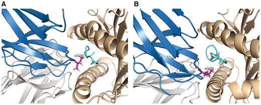
Differential effects of G28I to (A) AAG-binding and (B) ELA-binding revealed in iCFN structural models. TCR DMF5 α and β chains are shown in blue and gray cartoons, MHC Class I protein HLA-A2 in wheat cartoon, AAG/ELA peptide in cyan cartoon with N-terminal alanine/glutamate in sticks, and substitution I28 in purple sticks, respectively

4 Conclusions

We have developed, for the first time, an exact algorithm that is efficient for generic multistate protein design of unprecedented sizes to previous exact methods. The combinatorial optimization problem is formulated as coupled WCSPs where each WCSP corresponds to a substate design and is modeled by a CFN. The algorithm exploits novel bounds that can be quickly evaluated in the framework of CFN as well as joint consideration of substate CFNs that can quickly prune subtrees at the sequence, substate, and conformer levels with guarantee. Applications to XRCC1 binding affinity design and TCR specificity design prove that iCFN can be at least one to two orders of magnitude faster than COMETS with much less memory demand and can solve problems of sizes intangible to COMETS. Also, iCFN shows competitive accuracy compared with Rosetta in replicating experimental results. More importantly, our results suggest that the consideration of backbone global flexibility leads to more diverse solutions and higher sensitivity in protein design. And they provide new mechanistic insights into specificity in protein interactions. Future directions include parallelizing the algorithm and its codes on the architecture of graphics processing unit (GPU), incorporating more types of constraints seen in applications while allowing for more general objective functions and continuous rotamers, and deriving tighter yet economic bounds under the framework of CFN.

Acknowledgements

We thank the Bruce Donald group for the open-source OSPREY and Mark Hallen for the help on COMETS.

Funding

This project is in part supported by the National Science Foundation [CCF-1546278] and the National Institute of General Medical Sciences of the National Institutes of Health [R35GM124952]. M.K. had been supported by Texas A&M AgriLife under a Plant Bioinformatics Graduate Training Program (2015–17). Part of computing time is provided by the Texas A&M High Performance Research Computing.

Conflict of Interest: none declared.