piMGM: incorporating multi-source priors in mixed graphical models for learning disease networks

Abstract

Motivation

Learning probabilistic graphs over mixed data is an important way to combine gene expression and clinical disease data. Leveraging the existing, yet imperfect, information in pathway databases for mixed graphical model (MGM) learning is an understudied problem with tremendous potential applications in systems medicine, the problems of which often involve high-dimensional data.

Results

We present a new method, piMGM, which can learn with accuracy the structure of probabilistic graphs over mixed data by appropriately incorporating priors from multiple experts with different degrees of reliability. We show that piMGM accurately scores the reliability of prior information from a given expert even at low sample sizes. The reliability scores can be used to determine active pathways in healthy and disease samples. We tested piMGM on both simulated and real data from TCGA, and we found that its performance is not affected by unreliable priors. We demonstrate the applicability of piMGM by successfully using prior information to identify pathway components that are important in breast cancer and improve cancer subtype classification.

Availability and implementation

http://www.benoslab.pitt.edu/manatakisECCB2018.html

Supplementary information

Supplementary data are available at Bioinformatics online.

1 Introduction

We undoubtedly live in the era of data deluge. Massive amounts of data from different social and scientific fields are collected daily and stored in databases. Recently, many research efforts are focused on developing computationally efficient data analysis methods that can mine and reveal ‘hidden’ patterns, trends and associations in such large datasets. Probabilistic Graphical Models (PGMs) offer an attractive solution to this problem since they can: i) discover and elegantly represent (as a graph) the conditional (in)dependences between variables in a dataset; ii) estimate the joint probability distribution of the data (Koller and Friedman, 2009); information that can be used to develop predictive models of any variable in the network.

Many algorithms have been proposed for learning the underlying structure of PGMs (Koller and Friedman, 2009; Spirtes et al., 2000). One of the most popular is graphical lasso (glasso) (Friedman, 2008), which can quickly learn the underlying graph structure. Although glasso can only handle datasets of continuous variables, recent extensions can learn PGMs over mixed data (hereby referenced as Mixed Graphical Models—MGM) (Lee and Hastie, 2015; Sedgewick et al., 2016; Tsagris, 2017). MGMs are gaining popularity in biomedical research due to their ability to reveal complex associations among multimodal variables that jointly influence the disease or biological mechanism that generates the mixed dataset. However, due to the fact that most biomedical datasets are high-dimensional (i.e. small number of samples, large number of variables), their accuracy depends on the selection of regularization (sparsity) parameters, which control the sparsity of the graph (in terms of the number of edges) (Liu, 2010). Incorporating prior information during structure learning can significantly improve accuracy by biasing the computed structure on known biological associations.

During the last few years several methods have been proposed to incorporate prior information in graph structures learned over continuous variables. (Wang et al., 2013) proposed a modified glasso algorithm, named prior information dependent lasso (plasso), which aims to incorporate prior knowledge about the presence of the graph’s edges. To achieve this, the authors use two sparsity parameters: one for the edges for which no prior exists and one for those with prior information. To select the values of these parameters, the authors proposed two modified versions of the Bayesian Information Criterion. Both BIC versions introduce extra parameters (i.e. minimum average node degree and proportion of the true edges in the given prior information) where their values must be ‘guessed’ by the user. However, in real world applications, it is impossible for the user to know the ‘true’ values of these parameters, a fact that reduces the algorithm’s accuracy. Other modified versions of the glasso which can incorporate prior information into structure learning have been proposed by (Li and Jackson, 2015) and (Zuo et al., 2017). Their prior incorporation methods are based on the estimation of a confidence $p\times p$ matrix (where p is the number of variables) using prior information. The elements of this matrix take their values in [0-1], where a 1(0) indicates that there is (not) a connection between the corresponding pair of variables. To select the value of the glasso’s sparsity parameter, they propose the BIC and Cross-Validation (CV) methods. However, (Liu, 2010) in their seminal work have shown that although BIC and CV perform well in low dimensional data (i.e. small number of variables) they tend to perform poorly in high dimensional data.

We note that all these methods can incorporate prior information into graph structure learning over datasets with continuous only variables. In this paper we propose a new method, piMGM (prior incorporation Mixed Graphical Model), which incorporates prior information over mixed datasets, addresses the limitations of the aforementioned methods, and introduces the following unique aspects: (i) Incorporates prior information from multiple sources that may have different degrees of reliability. (ii) Introduces a novel probabilistic scheme to evaluate the reliability of each prior information source. (iii) Introduces a weighted scheme that fuses the multi-source information and represents it in a probabilistic way, which is used by the proposed prior information incorporation method. (iv) Introduces a novel score function for the selection of the regularization parameter values, which not only favors the incorporation of the most reliable prior information, but it also produces stable graphs (i.e. graphs insensitive to data variations). To the best of our knowledge this is the first method that attempts to incorporate prior information to graph structure learning over mixed data.

2 Materials and methods

2.1 Preliminaries

Suppose that we have a dataset $S$ of size $n\times p$ where $n$ is the number of samples and $p$ is the number of random variables. Using this dataset, the objective of a graph structure learning algorithm is to find a graph $G=\left(\mathcal{V},\mathcal{E}\right)$ that best represents the conditional dependences between the random variables. In graphical models, the nodes $\mathcal{V}$ of the graph, have a 1-1 correspondence to the random variables, and the presence of an edge ${\epsilon }_k\in \mathcal{E}$ indicates the conditional dependence relation between the $k^{th}$ pair of random variables. Throughout this paper, we assume that there is a fixed ordering over node pairs and we denote the set of corresponding edges as $\mathcal{E}=\left\{{\epsilon }_1,{\epsilon }_2,\dots ,{\epsilon }_K\right\}$ where $K=\frac{\left|\mathcal{V}\right|\left(\left|\mathcal{V}\right|-1\right)}{2}$ (number of edges in a fully connected graph with no self-loops). We assume that ${\epsilon }_k=1\left(0\right)$ if an edge is present (absent) between the kth $k^{th}$pair of nodes in the graph.

We denote the sources of prior information as $T=\left\{t_1,t_2,\dots ,t_R\right\}$⁠. The prior information of a source $t_r$ where $r=\left\{1,2,\dots ,R\right\}$ is given as a vector ${\vec{\mathcal{M}}}^{t_r}$ of size $K$⁠, where each of its elements $m_k^{t_r}$⁠, describes the probability of the corresponding edge (⁠${\epsilon }_k$⁠) to appear in the graph structure. For the edges with no available prior information about their presence, we assign a Null value to the corresponding vector elements. In general, each source $t_r\in T$ may provide information for a different subset of edges. $w{p}^{t_r}$ (with prior) and $n{p}^{t_r}$ (no prior) denote the set of edges for which the source $t_r$does or does not provide prior information, respectively. It holds that ⁠. Finally, we use $wp$ (⁠$np$⁠) to denote the set of edges for which we have (no) prior information.

2.2 Learning the structure of graphical models over mixed variables

In Sedgewick et al. (2016), the authors proposed a novel algorithm named CausalMGM which accurately learns the structure of graphical models over mixed variables (continuous and discrete), and it is an improvement over the work of Lee and Hastie (2015). CausalMGM’s novelties are: a) It utilizes edge type-specific regularization parameters $\left\{{\lambda }_{cc},{\lambda }_{cd},{\lambda }_{dd}\right\}$ for the model [see Equation (1)] for continuous-continuous, continuous-discrete and discrete-discrete edges, respectively, that control the sparsity (in terms of the number of edges) of the estimated graph structure. b) It proposes a computationally efficient subsampling method (StEPS) to select the value of these parameters which give the most stable graph structure, as high stability graphs should be closer to the true graphs.

Assume that we have p Gaussian variables $x$⁠, and q categorical $y$⁠. Equations (1)–(4) (Sedgewick et al., 2016) summarizes the MGM algorithm. The subscripts {1, 2, F} in Equation (1) denote the l₁, Euclidean and Frobenius norms respectively.${\beta }_{\omega \varphi }$ represents the interaction term between the continuous variables $x_{\omega }$ and $x_{\varphi }$⁠;${\rho }_{\omega \upsilon }$ represent the interaction term between continuous variable $x_{\omega }$ and discrete variable $y_{\upsilon }$⁠; ${\Upsilon }_{\zeta \upsilon }$ represents the interaction term between discrete variables $y_{\zeta }$ and $y_{\upsilon }$⁠. $\text{Θ}$ is shorthand for all the model parameters (i.e. $\left\{{\beta }_{\omega \varphi },{\alpha }_{\omega },{\rho }_{\omega \upsilon },{\Upsilon }_{\zeta \upsilon }\right\}$⁠). (Sedgewick et al., 2016) describes the MGM algorithm in detail.

Parameter estimation in the MGM model is done via:

$$argmi{n}_{\text{Θ}}\tilde{l}\left(\text{Θ}\right)+{\lambda }_{cc}{\displaystyle \sum }_{\varphi <\omega }{\left|{\beta }_{\omega \varphi }\right|}_1+{\lambda }_{cd}{\displaystyle \sum }_{\omega ,\upsilon }\Vert {\rho }_{\omega \upsilon }\Vert {}_2+{\lambda }_{dd}{\displaystyle \sum }_{\zeta <\upsilon }\Vert {\Upsilon }_{\zeta \upsilon }\Vert {}_F$$

(1)

where $\tilde{l}\left(\text{Θ}\right)$ is the negative log pseudo-likelihood:

$$\tilde{l}\left(\text{Θ}\right)=-{\displaystyle \sum }_{\omega =1}^p\log p\text{(}{x}_{\omega }\text{|}{x}_{\text{∖}\omega },y;\Theta )-{\displaystyle \sum }_{\zeta =1}^q\log p\text{(}{y}_{\zeta }\text{|}x,y_{\setminus \zeta };\Theta )$$

(2)

and $p\left(x,y;\Theta \right)$ is a pairwise Markov random field.

$$p\left(x,y;\Theta \right)\propto exp({\displaystyle \sum }_{\omega =1}^p{\displaystyle \sum }_{\varphi =1}^p-\frac{1}{2}{\beta }_{\omega \varphi }{x}_{\omega }{x}_{\varphi }+{\displaystyle \sum }_{\omega =1}^p{\alpha }_{\omega }{x}_{\omega }+{\displaystyle \sum }_{\omega =1}^p{\displaystyle \sum }_{\upsilon =1}^q{\rho }_{\omega \upsilon }\left(y_{\upsilon }\right)x_{\omega }+{\displaystyle \sum }_{\upsilon =1}^q{\displaystyle \sum }_{\zeta =1}^q{\Upsilon }_{\zeta \upsilon }\left(y_{\zeta },y_{\upsilon }\right))$$

(3)

2.3 Estimating prior information dependent MGM structures

In this section we present our new method, the prior information dependent MGM (piMGM), which appropriately combines the information from observational data with information provided by multiple sources (e.g. pathways, domain experts, etc.) with different confidence.

piMGM extends the framework of the original MGM [see Equation (1)] by replacing each of the norms in Equation (1) with two norms [see Equation (4)]: ${\lambda }_{xx}^{wp}$ and ${\lambda }_{xx}^{np}$ where $xx\in \{cc,cd,dd\}$ and wp and np designate the edge sets with prior or no prior information, respectively. This new scheme provides greater flexibility to the model, since it independently controls the sparsity of the corresponding types of graph’s edges (cc, cd and dd) for which we do or do not have prior information.

(4)

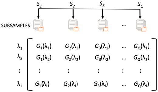
To estimate the values of the regularization parameters ${\lambda }_{xx}^{wp}$ and ${\lambda }_{xx}^{np}$⁠, we proposed the following procedure: We randomly draw $Q$ subsamples $\left\{S_1,S_2,\dots ,S_Q\right\}$ of size $b\left(1\le b\le n\right)$ from the dataset $S$ (Fig. 1). Unlike bootstrapping, each subsample is drawn without replacement. Since there is a total of $\left(\begin{array}{c}n\\ b\end{array}\right)$ different subsamples, $Q$ should satisfy $Q\le \left(\begin{array}{c}n\\ b\end{array}\right)$⁠. For each subsample $S_q$($q\in \left\{1,2,\dots ,Q\right\}$) we run the CausalMGM algorithm for a range of regularization parameter values $\Lambda =\left\{{\lambda }_1,{\lambda }_2,\dots ,{\lambda }_J\right\}$⁠. In order to reduce the time complexity of the method, we assume independence between the three different edge types (cc, cd, dd) as in Sedgewick et al. (2016), and so for each run we use the same value for all three regularization parameters ${\lambda }_{cc}={\lambda }_{cd}={\lambda }_{dd}$⁠. These runs generate $G_i$ graph structures, where $i\in \left\{1,2,\dots ,Q·J\right\}$ (Fig. 1). It is worth mentioning that CausalMGM runs $Q·J$ times independently, and therefore it can be easily parallelized for better efficiency.

Fig. 1.

The $Q·J$ graphical models. For each regularization parameter value λ, we estimate $Q$ graphical models’ structures

2.4 Data-driven estimation of the probabilities of presence of the graph edges

Using the graph structures that have been estimated using the regularization parameter values ${\lambda }_j\in \Lambda$ (see Fig. 1), we calculate the probability of presence of an edge ${\epsilon }_k\in \mathcal{E}$ as:

$${\mathcal{P}}_k^p=\frac{N_k}{Q·J}$$

(5)

where $N_k$ denotes the number of times ${\epsilon }_k$ appears in the $Q·J$ graphs.

2.4.1 Selecting regularization parameters ${\text{λ}}_{\text{xx}}^{\text{np}}$ for the edges with no prior

For each regularization parameter value ${\lambda }_j\in \Lambda$ we have estimated $Q$ graphs (Fig. 1). Using the structures of the $Q$ graphs, for each edge ${\epsilon }_k\in \mathcal{E}$⁠, we count the number of times, $z_k^{{\lambda }_j}\le Q$⁠, that ${\epsilon }_k$ appears in the $Q$ graphs. We assume $z_k^{{\lambda }_j}$ follows the Binomial distribution $B\left(Q,{\mathcal{P}}_k^p\right)$⁠, where ${\mathcal{P}}_k^p$ is the probability for edge ${\epsilon }_k$ to appear in a graph structure, and we calculate the probability ${\theta }_k^{{\lambda }_j}$ for edge ${\epsilon }_k$ to appear exactly $z_k^{{\lambda }_j}$times in the $Q$ graphs.

$${\theta }_k^{{\lambda }_j}=\left(\begin{array}{c}Q\\ z_k^{{\lambda }_j}\end{array}\right)·{\left({\mathcal{P}}_k^p\right)}^{z_k^{{\lambda }_j}}·{\left(1-{\mathcal{P}}_k^p\right)}^{Q-z_k^{{\lambda }_j}}$$

(6)

The higher the ${\theta }_k^{{\lambda }_j}$⁠, the better the regularization parameter ${\lambda }_j$‘explains’ the presence of the edge ${\epsilon }_k$ in the $Q$ graphs. Next, for each edge ${\epsilon }_k\in np$⁠, we calculate the relative frequency of its presence in the $Q$ graphs as follows:

$$f_k^{{\lambda }_j}=\frac{z_k^{{\lambda }_j}}{Q}$$

(7)

Using the $f_k^{{\lambda }_j}$ we then calculate,

$$g_k^{{\lambda }_j}=4·f_k^{{\lambda }_j}·\left(1-f_k^{{\lambda }_j}\right)$$

where

$$0\le g_k^{{\lambda }_j}\le 1$$

(8)

The algebraic expression in Equation (8) allows us to answer the following question for each edge ${\epsilon }_k\in np$⁠: ‘how often do the$Q$graphs disagree on the presence of${\epsilon }_k$?’ Therefore, $g_k^{{\lambda }_j}$ can be considered as a measure of instability for an edge ${\epsilon }_k$ in the $Q$ graphs (Liu, 2010).

After applying this procedure for all edges ${\epsilon }_k\in np$⁠, we calculate for each ${\lambda }_j\in \Lambda$ the following score:

$$scor{e}_{np}^{{\lambda }_j}={\displaystyle \sum }_{k=1}^{\left|np\right|}{\theta }_k^{{\lambda }_j}·\left(1-g_k^{{\lambda }_j}\right)$$

(9)

We select as ${\lambda }_{xx}^{np}$ the ${\lambda }_j\in \Lambda$ that maximizes the score function [Equation (9)]. This selection is justified if we observe that the value of the score function increases with an increase in the probabilities ${\theta }_k^{{\lambda }_j}$⁠, and decreases with an increase in the instabilities $g_k^{{\lambda }_j}$⁠. Therefore, the $\lambda$ that maximizes the score function defines a stable graph structure that ‘best explains’ the presence of the edges for which no prior information exists.

2.4.2 Selecting regularization parameters ${\text{λ}}_{\mathit{\text{xx}}}^{\mathit{\text{wp}}}$ for the edges with priors

In this section we present the selection procedure of the regularization parameters ${\lambda }_{xx}^{wp}$⁠, which control the incorporation of the prior information to the graphical model. First, we present the simplest case, where the prior information is provided by a single source $\left(t_1\right)$⁠, and then we continue with the general case, where multiple sources $T=\left\{t_1,t_2,\dots ,t_R\right\}$⁠, provide information about different subsets of edges $\left\{w{p}^{t_1},w{p}^{t_2},\dots ,w{p}^{t_R}\right\}$ when each source may have a different degree of reliability for the given dataset. For example, if we consider the KEGG pathways as different sources of prior information, then not all pathways are expected to be active (relevant) in a given gene expression dataset. Thus, the information included in the ‘irrelevant’ pathways will be ‘unreliable’ for this dataset.

Quantifying reliability of the prior information source(s): The probability $m_k^{t_r}$ (see Section 2.1) can be used to answer the question ‘how many times edge${\epsilon }_k$is expected to appear in$Q$graphs?’ In our case, for each ${\lambda }_j\in \Lambda$ we have $Q$ graphs and therefore the answer is:

$${\psi }_k^{t_r}=m_k^{t_r}·Q$$

(10)

The estimated probability of presence ${\mathcal{P}}_k^p$ [see equation (5)] of an edge ${\epsilon }_k\in w{p}^{t_r}$⁠, allows us to answer the same question. As discussed in Section 2.4.1, we assume that the number of times where an edge ${\epsilon }_k\in w{p}^{t_r}$ will appear across the $Q$ graphs is described by a Binomial distribution $B\left(Q,{\mathcal{P}}_k^p\right)$⁠. It has been proven that Normal distributions are very good approximations to Binomial distributions (Papoulis and Pillai, 2002). Therefore, to make our calculations computationally tractable, we approximate the corresponding Binomial distributions with normal distributions ${\mathcal{D}}_k=\mathcal{N}\left({\mu }_k^d,Va{r}_k^d\right)$ with parameters:

$$\begin{array}{c}{\mu }_k^d={\mathcal{P}}_k^p·Q\\ Va{r}_k^d={\mathcal{P}}_k^p·\left(1-{\mathcal{P}}_k^p\right)·Q\end{array}$$

(11)

Using ${\psi }_k^{t_r}$ and ${\mu }_k^d$⁠, we calculate:

$${\tau }^{t_r}=\frac{{{\displaystyle \sum }}_{k=1}^{\left|w{p}^{t_r}\right|}\left|{\psi }_k^{t_r}-{\mu }_k^d\right|}{\left|w{p}^{t_r}\right|}$$

(12)

Equation (12) measures the confidence we have on the source $t_r$⁠. More specifically, the larger the ${\tau }^{t_r}$ the less ‘confident’ we are about source $t_r$⁠. For the derivation of this formula, we assumed that the estimations ${\psi }_k^{t_r}$ of the source $t_r$⁠, should be similar to the estimations ${\mu }_k^d$⁠, which are derived from the data (i.e. the $Q·J$ graphs, Fig. 1).

However, prior information datasets may inform about different numbers of edges, which can affect the value of $\tau$⁠. For example, having prior information about the presence of only three edges may match the edges learned by a graphical model just by chance, even if this prior information is not well represented in the data (i.e. unreliable prior). To mitigate this, we learn an empirical null distribution similarly to GSEA (Subramanian et al., 2005). Given a prior source (e.g. a pathway) $t_r$ with $\left|w{p}^{t_r}\right|$ edges, we randomly permute the labels of the nodes in these edges (randomly select two other nodes to be in the edge) $N=10\hspace{0.17em}000$ times to produce a distribution of random pathways of equal size. For each pathway $r$ in this distribution, we compute ${\tau }^{t_r}$ exactly as specified in Equation (12). Then, the empirical P-value of the prior $t_r$ is the percentage of values in the null distribution greater than ${\tau }^{t_r}$⁠. To accurately measure ${\tau }^{t_r}$independently of the size of the prior, we normalize ${\tau }^{t_r}$ by dividing by the mean of the empirical null distribution. With this, P-value we can quantify whether we believe a prior source is well represented by the system under study.

Using Equations (10) and (12), we can model the prior information of a source $t_r$⁠, with a normal distribution ${\mathcal{U}}_k^{t_r}=\mathcal{N}\left({\psi }_k^{t_r},{\left({\tau }^{t_r}\right)}^2\right)$⁠, which describes the number of times where an edge ${\epsilon }_k\in w{p}^{t_r}$ is expected to appear in $Q$ graphs. Note that if more than one source of prior information is available (⁠$T=\left\{t_1,t_2,\dots ,t_R\right\}$⁠), then each source is modeled by a different normal distribution ${\mathcal{U}}_k^{t_i}$ (⁠$i=\left\{1,2,\dots ,R\right\}$⁠).

Selecting  ${\mathit{\lambda }}_{\mathit{xx}}^{\mathit{wp}}$  using prior information from a single source: If we have a single source of prior information (⁠$t_1$⁠), then for each edge ${\epsilon }_k\in wp$ we estimate two normal distributions: ${\mathcal{D}}_k=\mathcal{N}\left({\mu }_k^d,Va{r}_k^d\right)$⁠, which is estimated from the data; and ${\mathcal{U}}_k^{t_1}=\mathcal{N}\left({\psi }_k^{t_1},{\left({\tau }^{{\text{t}}_1}\right)}^2\right)$ which constitutes the $t_1$ prior information. By applying Bayes theorem, it can be proved (Bromiley) that since the prior ${\mathcal{U}}_k^{t_1}$ and the likelihood ${\mathcal{D}}_k$ are both Normal distributions, the posterior will also be Normal $\mathcal{N}\left({\mu }_k^{\text{*}},Va{r}_k^{\text{*}}\right)$ with parameters given by the following closed form expressions:

$${\mu }_k^{\text{*}}=\frac{{\mu }_k^d·{\left({\tau }^{t_1}\right)}^2+{\psi }_k^{t_1}·Va{r}_k^d}{{\left({\tau }^{t_1}\right)}^2+Va{r}_k^d},Va{r}_k^{\text{*}}=\frac{{\left({\tau }^{t_1}\right)}^2·Va{r}_k^d}{{\left({\tau }^{t_1}\right)}^2+Va{r}_k^d}$$

(13)

The posterior distribution $\mathcal{N}\left({\mu }_k^{\text{*}},Va{r}_k^{\text{*}}\right)$ is derived from the fusion of the information provided by source $t_1$ (prior information) and the data, and describes our updated ‘belief’ about the probability of an edge ${\epsilon }_k\in wp$ to appear a specific number of times in the $Q$ estimated graph structures.

For each regularization parameter value ${\lambda }_j\in \Lambda$ we have estimated $Q$ graphs (see Fig. 1). For each edge ${\epsilon }_k\in wp$⁠, we count the number of times $z_k^{{\lambda }_j}\le Q$ that it appears in the $Q$ graphs. From the corresponding posterior distributions, we can calculate for each edge ${\epsilon }_k\in wp$⁠, the probability ${\theta }_k^{{\lambda }_j}$⁠, to appear exactly $z_k^{{\lambda }_j}$ times in the $Q$ graphs

$${\theta }_k^{{\lambda }_j}=\underset{z_k^{{\lambda }_j}-\varepsilon }{\overset{z_k^{{\lambda }_j}+\varepsilon }{{\displaystyle \int }}}\mathcal{N}\left(x|{\mu }_k^{\text{*}},Va{r}_k^{\text{*}}\right)dx$$

(14)

where ɛ is an arbitrarily small positive quantity.

Using Equations (7) and (8) we calculate for each edge in ${\epsilon }_k\in wp$⁠, the relative frequency $f_k^{{\lambda }_j}$ of its presence in the $Q$ graphs, and its corresponding instability $g_k^{{\lambda }_j}$⁠. After applying this procedure for all edges ${\epsilon }_k\in wp$ we calculate for each ${\lambda }_j\in \Lambda$ the following score:

$$scor{e}_{wp}^{{\lambda }_j}={\displaystyle \sum }_{k=1}^{\left|wp\right|}{\theta }_k^{{\lambda }_j}·\left(1-g_k^{{\lambda }_j}\right)$$

(15)

We select as ${\lambda }_{xx}^{wp}$ the value of ${\lambda }_j\in \Lambda$ where the score function takes its maximum value. The justification of this selection is similar to the one provided in Section 2.4.1.

Selecting  ${\mathit{\lambda }}_{\mathit{xx}}^{\mathit{wp}}$  using prior information from multiple sources: In this section we present the selection procedure of ${\lambda }_{xx}^{wp}$ when prior information is provided by multiple sources $T=\left\{t_1,t_2,\dots ,t_R\right\}$⁠. Using Equations (10)–(12) we can estimate for each source $t_r\in T$ the normal distributions ${\mathcal{U}}_k^{t_r}$ that correspond to the edges ${\epsilon }_k\in w{p}^{t_r}$⁠. For each edge ${\epsilon }_k$ we have $\left|T_k\right|\le \left|T\right|$ normal distributions that were extracted by the information of the sources $T_k\subseteq T$ that contain prior information for edge ${\epsilon }_k$⁠.

Similar to the single source case, for each edge ${\epsilon }_k\in wp$ we estimate the following normal distributions: ${\mathcal{D}}_k=\mathcal{N}\left({\mu }_k^d,Va{r}_k^d\right)$ from the data; and $\left|T_k\right|$ normal distributions ${\mathcal{U}}_k^{t_r}=\mathcal{N}\left({\psi }_k^{t_r},{\left({\tau }^{t_r}\right)}^2\right)$⁠, which are estimated using the prior information of the sources $t_r\in T_k$⁠. To combine their information, we propose the following procedure:

First, we calculate the mixture of the $\left|T_k\right|$ normal distributions [black curve in Fig. 2a]

$${\Phi }_k\left(x\right)={\displaystyle \sum }_{i=1}^{\left|T_k\right|}{w}^{t_i}·\mathcal{N}\left({\psi }_k^{t_r},{\left({\tau }^{t_r}\right)}^2\right)$$

(16)

Fig. 2.

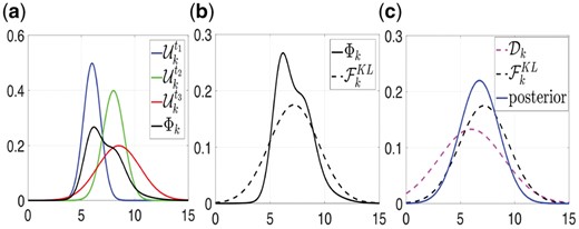
(a–c) The steps of the proposed information fusion method. (a) The prior information (normal distribution $\left\{{\mathcal{U}}_k^{t_1},{\mathcal{U}}_k^{t_2},{\mathcal{U}}_k^{t_3}\right\}$⁠) of the 3 sources $(\left\{t_1,t_2,t_3\right\}$- blue, green and red curves) and their corresponding mixture ${\Phi }_k$ (black curve). (b) The normal distribution ${\mathcal{F}}_k^{\text{KL}}$ (black dashed curve) that has minimum Kullback-Leibler divergence from the mixture ${\Phi }_k$(black continuous curve). (c) The posterior distribution which consists of the information fusion of the probability distribution ${\mathcal{D}}_k$ and the ${\mathcal{F}}_k^{\text{KL}}$(see text for details)

To calculate the mixture weights $w^{t_i}$⁠, we apply the following expressions:

$$w^{t_i}=\frac{a^{t_i}}{{{\displaystyle \sum }}_{i=1}^{\left|T_k\right|}{a}^{t_i}}\mathrm{where}{a}^{t_i}=\frac{{{\displaystyle \sum }}_{i=1}^{\left|T_k\right|}{\tau }^{t_i}}{{\tau }^{t_i}}$$

(17)

For the calculation of the weights (⁠$w^{t_i}$⁠), we use the assumption that the normal distributions with the smaller variances ${\left({\tau }^{t_i}\right)}^2$ should be trusted more. Note that ${\displaystyle \sum }_{i=1}^{\left|T_k\right|}{w}^{t_i}=1$⁠. Next, by applying variational calculus, we approximate the Gaussian mixture ${\Phi }_k\left(x\right)$ using a single normal distribution ${\mathcal{F}}_k^{\text{KL}}=\mathcal{N}\left({\mu }_k^{KL},Va{r}_k^{KL}\right)$ which minimizes the Kullback-Leibler (KL) discrimination (maximizes the similarity) from the Gaussian mixture. The parameters of the normal distribution ${\mathcal{F}}_k^{\text{KL}}$ are calculated using the following analytical algebraic expressions (Runnalls, 2007):

$${\mu }_k^{KL}={\displaystyle \sum }_{i=1}^{\left|T_k\right|}{w}^{t_i}·{\psi }_k^{t_{\text{i}}}$$

(18)

$$Va{r}_k^{KL}={\displaystyle \sum }_{i=1}^{\left|T_k\right|}{w}^{t_i}·\left({\left({\tau }^{t_i}\right)}^2+{\left({\mu }_k^{KL}-{\psi }_k^{t_{\text{i}}}\right)}^2\right)$$

(19)

After applying this procedure for all edges ${\epsilon }_k\in wp$ we have 2 normal distributions for each edge ${\epsilon }_k,$ a) the ${\mathcal{D}}_k=\mathcal{N}\left({\mu }_{\text{k}}^d,Va{r}_k^d\right)$⁠, which is estimated using the given dataset [pink dashed curve in Fig. 2c], and b) the distribution ${\mathcal{F}}_k^{\text{KL}}=\mathcal{N}\left({\mu }_k^{KL},Va{r}_k^{KL}\right)$ [black dashed curve in Fig. 2c]. Thus, for each edge ${\epsilon }_k\in wp$⁠, the parameters of the corresponding posterior distribution $\mathcal{N}\left({\mu }_k^{\text{*}},Va{r}_k^{\text{*}}\right)$ can be calculated using the expressions in Equation (13). Next, using Equations (14) and (15) we select the corresponding regularization parameter ${\lambda }_{xx}^{wp}$ as described in the single source case.

2.4.3 Limiting the selection range of the regularization parameters

In this section we propose a procedure that limits the selection range $\Lambda$ of the regularization parameters values, which help us to further improve the estimation of the graph structure. In many real world applications (e.g. biological, clinical, etc.) we expect the underlying graphical structures (e.g. gene networks) to be sparse (Wang et al., 2013). Our method exploits this by limiting the selection range (⁠${\Lambda }^{\text{*}}\subseteq \Lambda$⁠) of regularization parameter values such as to avoid the selection of parameter values that result in very dense or very sparse graph structures.

For each regularization parameter value $\left\{{\lambda }_1,{\lambda }_2,\dots ,{\lambda }_J\right\}$ we calculate the average number of edges that appear across the $Q$ graph structures, estimated using the $S_q$ (⁠$q\in \left\{1,2,\dots ,Q\right\}$⁠) subsamples (see Fig. 1). In Figure 3 each red circle corresponds to the average number of edges that appear across the $Q$ graphs for a specific regularization parameter value. The curve formed by the red circles in Figure 3a indicates that as $\lambda$ increases (x-axis) the number of edges (y-axis) in the graphs monotonically decreases. Note that for small (large) values of $\lambda$ the estimated graphs are almost fully connected (empty). Below we propose to use a new procedure to limit the selection range of the regularization parameter values.

Fig. 3.

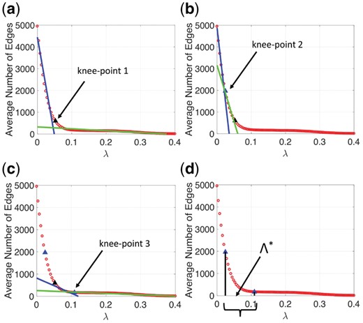
(a–c) The ‘knee-points’ and the estimated lines (blue and green) that minimize the corresponding sums of fit errors. (d) The new range of the regularization parameter values ${\Lambda }^{\text{*}}\subseteq \Lambda$ determined by the ‘knee-points’ 2 and 3 on the x-axis (black line segments)

We traverse the monotonically decreasing curve one point at a time (‘current point’) and fit two lines. The first line [blue line in Fig. 3a] is fitted to the points that belong on the left side of the ‘current point’ and the second line [green line in Fig. 3a] is fitted to the points that belong on the right side of the ‘current point’. The ‘current point’ that corresponds to the minimum sum of the corresponding lines’ fit errors becomes a ‘knee-point’ [see ‘knee-point’ 1 in Fig. 3a]. We apply this procedure to the points that are located on the left and right side of ‘knee-point’ 1 [see Fig. 3b and c] and we determine the ‘knee-point’ 2 and 3 respectively. The projections of the ‘knee-points’ 2 and 3 on the x-axis [see Fig. 3d], determine the ‘new’ selection range (⁠${\Lambda }^{\text{*}}=\left\{{\lambda }_1,{\lambda }_2,\dots ,{\lambda }_{J^{\text{*}}}\right\}\subseteq \Lambda$⁠) of the regularization parameter values which will be used by our regularization parameter selection method (see Section 2.4).

3 Results

To demonstrate the value of piMGM we used simulated and real data. In the latter case, we also address two important biological problems: i) pathway scoring on expression datasets and ii) network structure inference for understanding of genomic drivers of disease subtype.

3.1 Description of data sources

Simulated data. Simulated datasets of varying sizes were generated using the Lee and Hastie simulation method from Tetrad VI (http://www.phil.cmu.edu/tetrad/). First, a Directed Acyclic Graph (DAG) was generated uniformly at random with number of edges equal to the number of nodes. Each node was randomly assigned to be a continuous or categorical variable with equal probability. This DAG was parameterized with random edge weights in the range:

[−1.5, −0.5], [0.5, 1.5]. Independent samples were generated from this parameterized graph to produce a final dataset, according to the model from Lee and Hastie (2015). To compare the estimated graph learned by piMGM, the DAG was converted to its equivalent ‘moralized’ undirected version, which maintains the independence relationships present in the original DAG (Cowell, 1999).

Prior sources were generated based on the ground truth DAG using two different methods depending on whether we wanted to evaluate learning of the full network or scoring the prior sources (also called ‘pathways’ here to highlight their relevance to biological pathways in gene expression data). Specifically, for the pathway experiments: we defined a ‘pathway’ i as a random selection of E_i edges, where E_i is in the range [10, 2N] and N is the number of edges in the data generating moralized graph. We then randomly selected T_i edges from the ground truth graph to include in the pathway, where. T_i is randomly selected from the range: [1, $min(E_i,\text{ N})$]. Thus, the reliability of pathway $i$ is $T_i/E_i$⁠, which measures what percent of a pathway’s edges are present in the data generating graph. Finally, we randomly selected E_i-T_i ‘false’ edges from all edges not in the data generating graph. These pathways were given as ‘hard priors’ which means that the prior information given by a pathway only contained the values null and 1 corresponding to the absence or presence of an edge in the pathway, respectively.

For the full network inference experiments, it was assumed that all prior sources provide information about the same edges, but with different reliability, to test the ability of piMGM to successfully synthesize prior information from multiple sources. We tested cases where the sources only provide information for the true edges in the ground truth graph and for edges uniformly at random. The number of edges provided, and the number of experts were experimentally controlled. The edges for which the experts give prior information were determined randomly, and the information itself was a ‘soft prior’ with a real numbered value ranging from (0.6, 1) for a reliable source, and from (0, 1) for an unreliable source; in contrast to the ‘hard priors’ from the previous pathway experiments.

Biological data. We used the TCGA-BRCA RNA-Seq expression dataset to demonstrate the applicability of piMGM. This data included gene expression measurements from 800 breast tumor samples and 95 matched normal samples. Prior information consisted of 33 Kyoto Encyclopedia of Genes and Genomes (KEGG) pathways (Kanehisa and Goto, 2000), which were selected by the same criteria as a related pathway enrichment method (Ma et al., 2016), but excluding those with fewer than 10 expressed genes or fewer than 20 gene–gene interactions. The gene–gene interactions encoded in each pathway were used as a ‘hard prior’ with a value of 1 if the edge existed in the pathway, and no information otherwise. 645 genes were included in the final dataset, consisting of the union of the genes in the 33 pathways, excluding 2735 consistently lowly expressed genes or those without a variance of at least 0.5.

To evaluate the usefulness of full network inference for classification, breast cancer subtype information for each tumor sample was obtained from Jiang et al. (2016). This determination was used as a ground truth for classification experiments, and the fifty genes commonly used to compute this classification on microarray data, Prediction Analysis of Microarray 50 (PAM50) was used as a prior information source. In this case, the edges between each gene in the PAM50 list and the categorical variable denoting subtype was given a prior probability of 1, while all other edges had no prior information.

3.2 piMGM for pathway activation assessment

We first evaluate how well piMGM determines the state of activation of given pathways using both simulated and real data.

3.2.1 piMGM correctly estimates the reliability of pathways

Figure 4 presents the results of applying piMGM on 25 simulated datasets with 100 variables each, 15 pathways for prior information, and 200 samples. The figure demonstrates the strong inverse correlation between the predicted deviance [Equation (12)] of each simulated pathway from the ground truth and its reliability score that piMGM calculated. The major outliers from the trendline are those pathways that provide information about relatively few gene–gene interaction edges. This is because if a pathway has few interactions, they might match spurious correlations in the dataset by chance. Thus, it is prudent to consider both the reliability score of the pathway as well as its P-value to determine its reliability. On a graph by graph basis, the mean correlation between τ and the reliability score across all 25 datasets was 0.992 (±0.006), further confirming the accuracy of the piMGM model for each individual dataset.

Fig. 4.

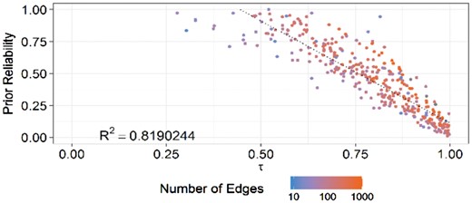
Association between the true reliability of priors (experts) and the deviance (τ) of the data from the priors as calculated by piMGM

3.2.2 Identifying gene pathways associated with breast cancer subtypes

As a first application of piMGM on biological data, we used it to identify de-regulated pathways in breast cancer patients from TCGA. In this application, we used the pathways as ‘experts’ and we scored their ‘reliability’ on tumor and normal samples. ‘Reliable’ pathways are those that are active in the given sample dataset (low P-value; Section 2.4.2), and ‘unreliable’ are those that are not. We selected 33 pathways from KEGG for this test, as we describe in the Section 2.

piMGM found eight of the 33 pathways to be differentially regulated (FDR-corrected P-value < 0.1) between receptor positive (Luminal A and B subtypes) and receptor negative (HER2 and Triple-Negative) subtypes (Table 1). Five of the eight pathways were also found to be differentially expressed by a related method, NetGSA, so we further examined the three remaining pathways to understand what piMGM found mechanistically.

Table 1.

Differentially regulated pathways by receptor status (positive: Luminal A and B; negative: HER2, triple negative) in Breast Cancer (FDR < 0.1)

Pathway	P-value (+)	P-value (−)	Reference
Glutathione metabolism	0.507	0.091	Lien et al. (2016)
Glycolysis	0.000	0.129	Schramm et al. (2010)
Neurotrophin signaling	0.702	0.074	Patani et al. (2011)
Notch signaling	0.000	0.223	Hossain et al. (2017)
Pentose phosphate	0.025	0.239	Cha et al. (2017)
B Cell Receptor signaling	0.141	0.004	Hill et al. (2011)
Insulin signaling	0.098	0.384	(see text)
T cell receptor signaling	0.507	0.058	(see text)

Note: Pathways in italics found by piMGM but not NetGSA. The significance of the bold values is an FDR < 0.1.

We found that both the T and B cell receptor signaling pathways shared a common subnetwork that was driving their identification by piMGM as significant. This network included genes AKT3, PIK3CA, PIK3CD and PIK3R1 (Fig. 5, left), all of which are genes of significance in cancer. Several studies have found changes in the regulation of AKT3 in receptor negative breast cancer (Chin et al., 2014; Nakatani et al., 1999) and one recent study has found changes in expression of PI3K/Akt across receptor subtypes (Cizkova et al., 2013), consistent with our identified subnetwork An interesting finding from this pathway is that the direct connection between PIK3CA and AKT3 is more present in receptor negative tumors. PIK3CA is an oncogene whose aberrant activation results in AKT3 activation which can lead to uncontrolled cell proliferation and tumorigenesis (Hernandez-Aya and Gonzalez-Angulo, 2011). It is possible that this subnetwork elucidates distinct mechanisms of AKT3 overactivation in different breast cancer subtypes. piMGM also identified a NFATC1 subnetwork of T cell receptor pathway as critical for breast cancer development (Fig. 5, right). NFAT1 is a nuclear factor that alters T-cell transcription in response to T-cell receptor stimulation, but NFAT1 mRNA is also found in breast tissue (Safran et al., 2010). A recent study found that the NFAT1 pathway was active in triple negative breast cancer but not in other subtypes, and that the pathway was critical for metastasis and tumorigenesis (Quang et al., 2015). Though KEGG labels these pathways as lymphocyte related pathways (T and B cells), the reason these pathways were found to be differentially regulated was due to the subcomponents critical to breast cancer progression in different subtypes.

Fig. 5.

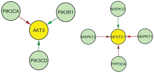
Edge differences between receptor positive (luminal A and B) and receptor negative (HER2, triple negative) breast tumor samples for a common sub-network of the T cell and B cell receptor signaling pathways (left) and the T cell receptor signaling pathway (right). Red edges are those that are more stable in receptor positive breast cancer, while green refers to receptor negative breast cancer. AKT3 and NFATC1 regulation appear to be driving the change between these phenotypic groups

The third pathway not corroborated by NetGSA was the insulin signaling pathway. Studies have shown that estrogen receptor positive cells can have increased proliferation in the presence of estrogen due to upregulation of the insulin receptor (IRS1), which binds insulin growth factor (IGF) (Molloy et al., 2000). Several of the most divergent connections found by piMGM involve IRS1 in the insulin signaling pathway (Supplementary Material).

All eight differentially regulated pathways appear to have an established relationship to breast tumor subtype. piMGM not only identified them as significant, but it also identified which parts of them are the most significant in breast cancer subtyping (Fig. 5), thus pointing to the mechanisms that influence this subtyping. Follow up studies can further investigate the specific mechanisms implied by piMGM networks. We should also note that piMGM tends to identify fewer differentially regulated pathways than conventional analysis techniques, but this is largely because piMGM uses stronger conditions than typical pathway enrichment methods. piMGM uses independence changes between genes while conventional enrichment methods ignore network connectivity and focus on gene expression changes. Individual gene expression changes may be related to established pathways, but independence relationships query the precise network information stored in KEGG pathways to determine differential regulation.

3.3 piMGM for full network inference

Next, we present piMGM results on simulated and biological data for inference of the full network structure on datasets with mixed continuous and categorical variables. Again, the prior information sets (i.e. ‘experts’) can have different degrees of reliability.

3.3.1 piMGM learns accurate networks despite unreliable priors

To evaluate the ability of piMGM to incorporate prior information, we compared piMGM with several baseline approaches on simulated data we generated as described in Section 2. We used four baseline methods for comparison (Fig. 6, left columns, 0% prior). STARS (Liu, 2010) is a network stability approach that tunes a single regularization parameter for MGM without prior information. STEPS is an extension of this approach that uses three regularization parameters, one for each edge type (Continuous-Continuous, Continuous-Discrete, Discrete-Discrete). The Oracle graph is MGM run with the set of three regularization parameters that maximize accuracy, and Oracle One λ is an equivalent approach using only one regularization parameter for the whole network.

Fig. 6.

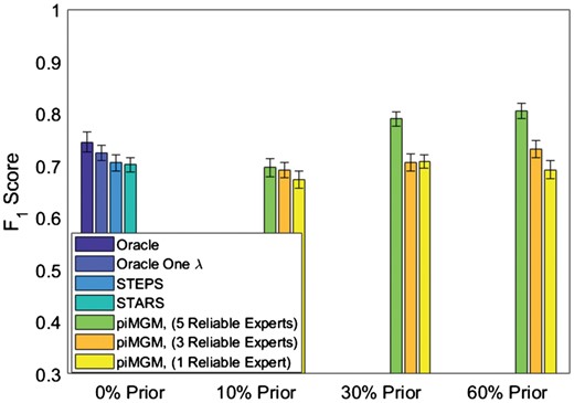
Accuracy of piMGM inferred networks vs. other approaches on simulated data with 100 variables, 500 samples and 5 prior sources. The datasets differ in the percent of edges with prior information (0, 10, 30, 60%) and the number of reliable priors (1, 3, 5 out of 5). The blue bars represent the F1 score accuracy of the baseline networks (no prior)

We compared the baseline results with piMGM runs with five prior information sources, varying both the percent of edges with prior information (10%, 30%, 60%) and the number of reliable experts among those 5 (reliable experts: 1, 3 or all 5). Figure 6 displays the amount of prior information (x axis) vs. the F1 score of the learned graph compared to the ground truth (moralized) graph. As expected, increase in the ratio of reliable to unreliable priors increases overall accuracy (F1 score) for all percentages of edges with prior information. We also see that in most cases the F1 score is not affected by unreliable priors even when 4 out of 5 experts are unreliable (Fig. 6, yellow bars; compared to STARS and STEPS methods with no prior). Interestingly, if prior information is available for 10% of edges, piMGM is equivalent to approaches with no priors, regardless of the reliability of the information sources. However, if 60% of edges have prior information, piMGM outperforms even the Oracle graph given that the prior information is somewhat reliable (P < 0.01). If the prior information is highly unreliable, with 30% prior, piMGM does not have degrading performance, and it maintains at least the quality that it would have had without any prior (P > 0.05). This is desirable in cases where prior information may or may not be well represented in the system under study. When ‘experts’ provide priors for edges that are not in the data generating graph the results are nearly identical (Supplementary Material).

3.3.2 Prior knowledge helps stabilize predictive models

Our final experiment evaluates the ability of piMGM to recover network structure from biomedical mixed data. Since ground truth for the whole network is difficult to come by in biological systems due to incomplete understanding of them, we evaluated our approach by determining how well the learned network can be used for a classification task. One of the advantages of graphical models is that you can use the variables that are connected to a target variable in the network (the Markov blanket, if the network is directed) to predict the target variable. Breast cancer consists of four subtypes with varying prognoses: triple negative, Luminal A, Luminal B and HER2. Using nested 10X cross validation, we tested the ability of our piMGM graphs to correctly classify the four subtypes. We compared classification accuracies on networks learned using four sets of priors: No prior information, five random sets of fifty genes each connected to the Subtype variable (Random Prior—unreliable), the PAM50 set of genes (PAM 50 Prior) and the same five random sets along with the PAM50 gene set (Both Priors). We ran piMGM with each of these sources as prior information and inferred a full network from data consisting of the 50 genes in PAM50 along with the genes used in Section 3.2.2. We then used the genes connected to the subtype variable as features in a multiclass logistic regression model.

We found that there is no significant difference in classification accuracy between each of the four models (Fig. 7, left columns). This means that piMGM is not affected by random (unreliable) priors even when they are the only source of information piMGM gets. On the other hand, incorporating appropriate prior information results into models that require significantly fewer features to achieve the same accuracy (Fig. 7, right columns). In addition, piMGM found the PAM50 gene set to be active in the BRCA dataset of tumor samples (P < 0.01) unlike the random gene sets (P > 0.1). piMGM does not have a reduction in classification performance when given a random prior source, further proving that this method is resilient to unreliable prior information sources on real data.

Fig. 7.

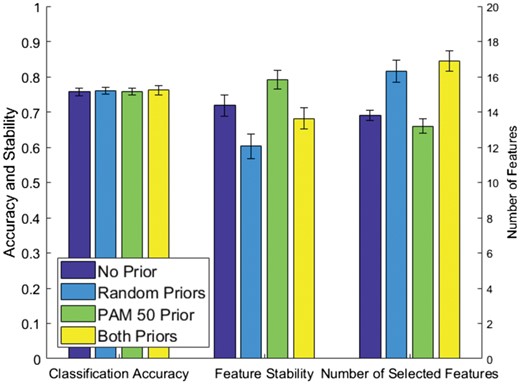
piMGM Network Inference to classify breast cancer subtypes with varying prior information. Performance is measured using classification accuracy and stability (y-axis left) and the number of features used in the model (y-axis right)

4 Discussion

We have presented a novel method to incorporate prior knowledge for learning mixed graphical models; and two applications of this method to genomic and clinical data. Our method, piMGM, which can incorporate multiple priors with varying degrees of reliability, consists of three steps, each of which presents a new algorithmic novelty. Step-1, we developed a novel reliability score [Equation (12)] that quantifies how well the prior information from a given expert fits the data. The reliability score has an interesting application: it can be used to assess whether a gene pathway is active in the data. Our analysis on TCGA data identified several previously known and novel pathways implicated in breast cancer. Step-2, we developed a novel method that uses the reliability score to weight and merge prior information from multiple experts into a single prior distribution for each edge. Step-3, we presented a new approach to incorporate prior information in the learning of probabilistic graphs over mixed data types. This method uses separate regularization parameters for edges with and without priors. The regularization parameters are also edge type specific to allow more flexibility and reduce false positive edges as we have shown in (Sedgewick et al., 2016). In simulated data we showed that piMGM is not affected by unreliable priors, and its performance increases with increasing amounts of prior information. When 60% of edges have informative (i.e. relatively reliable) priors, piMGM outperforms the Oracle graph without prior. The efficiency of piMGM in analyzing omics and clinical data was demonstrated in a classification example, where the variables surrounding the breast subtype variable in the learned graph were used in classification. We compared classification efficiencies of graphs learned with no priors, PAM50 genes, random priors and combination of PAM50 and random priors. We showed that the classification accuracy of piMGM is not affected by the inclusion of random priors (Fig. 7), but including PAM50 priors reduces the number of variables required for efficient classification. All parameters of piMGM can be ‘best’ selected using a subsampling procedure presented in Section 2.3, thus eliminating arbitrary choices. Furthermore, this procedure is parallelizable for increased efficiency.

To the best of our knowledge, this is the first method to incorporate unreliable prior information sources to infer a full network from mixed data and the first method to analyze pathway activation in single phenotype samples. We believe that piMGM is a valuable method that will help future analyses of datasets with mixed data types (continuous and discrete variables). In systems biology research, it will not only identify deregulated pathways, but it will also generate hypotheses about specific edges that are deregulated to guide intervention experiments.

Acknowledgements

We thank Prof. Peter Spirtes, Carnegie Mellon University, for critically reviewing a previous version of this manuscript. This work was supported by NIH through grants U01HL137159, R01LM012087 and T32CA082084).

Funding

This work was supported by the National Institutes of Health (NIH) under award numbers R01LM012087, U01HL137159 to Prof. Panayiotis V. Benos. Vineet K. Raghu was supported by a NIH training fellowship (T32CA082084). The content is solely the responsibility of the authors and does not necessarily represent the official views of the NIH.

Conflict of Interest: none declared.

Author notes

The authors wish it to be known that, in their opinion, Dimitris V. Manatakis and Vineet K. Raghu authors should be regarded as Joint First Authors.