Liquid-chromatography retention order prediction for metabolite identification

Abstract

Motivation

Liquid Chromatography (LC) followed by tandem Mass Spectrometry (MS/MS) is one of the predominant methods for metabolite identification. In recent years, machine learning has started to transform the analysis of tandem mass spectra and the identification of small molecules. In contrast, LC data is rarely used to improve metabolite identification, despite numerous published methods for retention time prediction using machine learning.

Results

We present a machine learning method for predicting the retention order of molecules; that is, the order in which molecules elute from the LC column. Our method has important advantages over previous approaches: We show that retention order is much better conserved between instruments than retention time. To this end, our method can be trained using retention time measurements from different LC systems and configurations without tedious pre-processing, significantly increasing the amount of available training data. Our experiments demonstrate that retention order prediction is an effective way to learn retention behaviour of molecules from heterogeneous retention time data. Finally, we demonstrate how retention order prediction and MS/MS-based scores can be combined for more accurate metabolite identifications when analyzing a complete LC-MS/MS run.

Availability and implementation

Implementation of the method is available at https://version.aalto.fi/gitlab/bache1/retention_order_prediction.git.

1 Introduction

In metabolomics, one of the most pressing challenges is the identification of the metabolites present in a sample. At present, the vast majority of metabolites in an untargeted metabolomics experiment are left unidentified; this is sometimes called the ‘dark matter’ of metabolism (Aksenov et al., 2017; da Silva et al., 2015). Liquid chromatography (LC) is widely used in untargeted metabolomics studies in combination with tandem mass spectrometry (MS/MS), due to the outstanding sensitivity of this combination and the applicability to a wide range of molecules. In short, LC separates metabolites by their retention time, MS separates the metabolites by their mass (per charge, m/z); finally, MS/MS selects a precursor mass, fragments the molecule and records masses of its fragments (Fig. 1). Retention times can be valuable orthogonal information (Hu et al., 2018; Ruttkies et al., 2016) for metabolite identification, e.g. by restricting the set of candidate identifications (Aicheler et al., 2015; Creek et al., 2011) or the distinction of diastereoisomers which have similar tandem mass spectra but different retention times (Stanstrup et al., 2015).

Fig. 1.

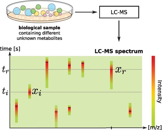
Schematic representation of retention times, MS, and MS/MS data in a metabolomics experiment. MS/MS spectra are measured at high-intensity peaks in the (retention time, mass per charge) space

In recent years, machine learning has arisen as a method to predict the metabolite identities from MS/MS spectra Allen et al., 2014; Brouard et al., 2016, 2017; Dührkop et al., 2015; Heinonen et al., 2012; Shen et al., 2014 and produced a step-change in metabolite identification accuracy (Schymanski et al., 2017). These methods are trained with a large number of reference spectra of single compounds and are effective in scoring and ranking the candidate molecular structures. However, these methods currently do not make use of retention time information. This is partly explained by the challenges posed by the available data: First, publicly available datasets are system specific and relatively small. Secondly, retention times are poorly comparable between different chromatographic systems and configurations, e.g. systems operated by different laboratories. Translating retention times of one system to another corresponds to a non-linear mapping, which needs to be estimated for each pair of systems and configurations separately (Stanstrup et al., 2015).

Retention time prediction has been addressed in numerous publications over the last decades, see Heberger (2007); Kaliszan (2007) for reviews. Quantitative-Structure-Retention-Relationship (QSRR) models use machine learning to predict retention times from molecular structures. Physicochemical properties derived from the structure or molecular fingerprints are commonly used as features, and regression is commonly used as prediction model (Aicheler et al., 2015; Creek et al., 2011; Falchi et al., 2016). QSRR models are mostly trained for one particular target chromatographic system, and predictions can be made only for this system. Few approaches try to overcome this problem, for example, by including descriptors of the chromatographic system into the prediction model: D’Archivio et al. (2012) used the retention behavior of standard compounds for this purpose. However, this requires that in a particular target chromatographic system those compounds have been measured as well. A different approach are retention time projection methods, which establish mappings between the retention times of different chromatographic system. Predictions for new molecules in a particular target chromatographic system are restricted to those molecules which have been measured with another chromatographic system already (Stanstrup et al., 2015).

In this paper, we propose a new way to predict LC retention behaviour of molecules that overcomes the above limitations, and to use the predictions to improve metabolite identification in combination with an MS/MS based predictor (Fig. 2). Our proposed retention order prediction method belongs to the so called preference learning or learning to rank family (Elisseeff and Weston, 2002; Fürnkranz and Hüllermeier, 2011), where the goal is to predict the preference order or ranking of the objects. In our case, the prediction target is the order in which different molecules elute from the LC column. We learn from the retention time measurements of different chromatographic systems how pairs of molecules are generally ordered by the LC systems. Our framework predicts this retention order directly from molecular structure, and these predictions can be made for any chromatographic system without the need of first mapping the retention time to a common time scale. In the subsequent phase, the predicted retention orders are combined with the scored candidate lists output by an MS/MS-based predictor, in our case, IOKR (Brouard et al., 2016). Computing the combined score efficiently entails solving a shortest path problem using dynamic programming in a graph defined by the IOKR candidate lists sorted by the retention time and connected by edges reflecting the retention order prediction. In summary, the contributions of the paper are as follows:

• We introduce the concept of retention order prediction for LC, and provide a machine learning framework for learning retention orders of molecules.

• We introduce a dynamic programming methodology for integrating retention order and MS/MS based scores to jointly identify a set of metabolites arising, e.g. in a metabolomics experiment and show that the approach can significantly improve the metabolite identification accuracy.

• We show that counting fingerprints have superior performance in retention order prediction over standard binary fingerprints.

• We demonstrate that the retention order framework is able to benefit from retention time measurements arising from heterogeneous LC systems and configurations.

Fig. 2.

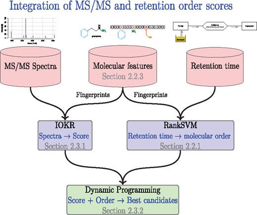
The flowchart showing the usage of retention time, MS/MS, and molecular property data sources to provide MS/MS based scores for candidate molecules and retention order predictions for pairs of molecules, as well as the dynamic programming module to integrate the two kind of predictors into a joint identification for a set of metabolites

2 Materials and methods

In this section, we first describe the methods used to learn the retention order of molecules. Subsequently, we present our framework for the integration of MS/MS based scores and predicted retention orders.

2.1 Notation

In this paper, we use the following notations: m denotes a molecule belonging to a set $\mathcal{M},x$ denotes a tandem mass spectrum belonging to a set $\mathcal{X}$ and $t\in {\mathbb{R}}_{+}$ denotes the retention time of a molecule. The molecules have been measured using different chromatographic systems belonging to the set $\text{S}$⁠. We define the set $S\subseteq \text{S}$ as the subset of chromatographic systems contained in our training data.

We consider two kernel functions $k_m:\mathcal{M}\times \mathcal{M}\to \mathbb{R}$ and $k_x:\mathcal{X}\times \mathcal{X}\to \mathbb{R}$ that measure, respectively, the similarity between molecules and similarity between MS/MS spectra. The kernel $k_m$ (resp. $k_x$⁠) is associated with a feature space ${\mathcal{F}}_m$ (resp. ${\mathcal{F}}_x$⁠) and a feature map $\phi :\mathcal{M}\to {\mathcal{F}}_m$ (resp. $\text{ϕ}:\mathcal{X}\to {\mathcal{F}}_x$⁠) that embeds molecules into the feature space ${\mathcal{F}}_m$ (resp. ${\mathcal{F}}_x$⁠). Through the next sections we use the following shortcuts: ${\phi }_i=\phi (m_i)$ and ${\text{ϕ}}_i=\text{ϕ}(x_i)$⁠.

2.2 Predicting retention behaviour of molecules with machine learning

In this section, we describe two methods that can be used to predict the retention behaviour (retention time or retention order) of molecules in the LC column. For retention order prediction, we introduce the use of RankSVM (Elisseeff and Weston, 2002; Joachims, 2002) method and for retention time prediction we apply the Support Vector Regression method (SVR; Smola and Schölkopf, 2004; Vapnik, 1995) which has already been used in that application by Aicheler et al. (2015).

2.2.1 Predicting retention order with ranking support vector machine (RankSVM)

RankSVM (Elisseeff and Weston, 2002) can be used to predict pairwise preferences between different objects and has been successfully applied in many order learning applications, e.g. in document ranking for search engines (Joachims, 2002). We use RankSVM to predict pairwise preferences between molecules. We define a molecule m_i as preferred over m_j if its retention time t_i is smaller than t_j, i.e. it m_i elutes before m_j from the chromatographic system. The set of pairwise preferences between molecules for each chromatographic system $s\in S$ can be defined as:

$$\mathcal{P}(s)=\{(i,j)|s_i=s_j=s,t_i<t_j\},$$

where s_i and s_j denote the systems used to, respectively, measure the molecules m_i and m_j. The union of pairwise preferences extracted from the whole training dataset is defined as:

$$\mathcal{P}={\displaystyle \underset{s\in S}{\cup }\mathcal{P}}(s),$$

(1)

and p is defined as $p=\left|\mathcal{P}\right|$⁠.

RankSVM learns a function $f:\mathcal{M}\times \mathcal{M}\to \{-1,1\}$ that predicts whether t_i < t_j given two molecules m_i and m_j. The values of this function f can be written as: $f(m_i,m_j)=\text{sign}(w^T(\phi (m_j)-\phi (m_i)))$⁠, where $\phi$ is a feature map embedding molecules to the feature space ${\mathcal{F}}_m$ and $w$ contains the feature weights to be learned.

The RankSVM solves the following optimization problem:

$$\begin{array}{l}\underset{w,\xi }{\min }\frac{1}{2}{w}^{T}w+C{\displaystyle \sum _{(i,j)\in \mathcal{P}}{\text{ξ}}_{ij}}\\ s.t.w^T({\phi }_j-{\phi }_i)\ge 1-{\text{ξ}}_{ij},\forall (i,j)\in \mathcal{P}\\ {\text{ξ}}_{ij}\ge 0,\forall (i,j)\in \mathcal{P},\end{array}$$

(2)

with C > 0 being a regularization parameter controlling the trade-off between fitting and regularization. By solving the Problem (2) we learn $w$ such that:

$$w^T{\phi }_i<w^T{\phi }_j,\text{if}(i,j)\in \mathcal{P}.$$

The dual formulation of the optimization problem (2) is the following:

$$\begin{array}{l}\underset{\alpha }{\max }-\frac{1}{2}{\alpha }^{T}Q\alpha +1^T\alpha \\ s.t.0\le {\text{α}}_{ij}\le C,\forall (i,j)\in \mathcal{P},\end{array}$$

with $\alpha \in {\mathbb{R}}^p,Q\in {\mathbb{R}}^{p\times p}$ and $1\in {\mathbb{R}}^p$ being a vector of ones. $Q$ is a pairwise kernel matrix defined as:

$$\begin{array}{l}{[Q]}_{(i,j),(u,v)}={({\phi }_j-{\phi }_i)}^T({\phi }_v-{\phi }_u)\\ ={\phi }_j^T{\phi }_v-{\phi }_j^T{\phi }_u-{\phi }_i^T{\phi }_v+{\phi }_i^T{\phi }_u.\end{array}$$

During the optimization we do not need to keep the whole $Q$ matrix in the memory. Instead, we can decompose the matrix as follows (Kuo et al., 2014):

$$Q=A{K}_m{A}^T,$$

where $K_m\in {\mathbb{R}}^{\ell \times \ell }$ is the kernel matrix associated with the kernel function $k_m$ and is defined as: ${[K_m]}_{i,j}={\phi }_i^T{\phi }_j$⁠, and $\ell$ corresponds to the number of molecular structures in the training dataset. The matrix $A\in {\mathbb{R}}^{p\times \ell }$ is defined as:

$${[A]}_{(i,j),·}=(0,\dots ,0,\underset{i.}{\underbrace{-1}},0,\dots ,0,\underset{j.}{\underbrace{+1}},0,\dots ,0),$$

and can be represented as sparse matrix during the optimization.

2.2.2 Predicting retention times with support vector regression (SVR)

We compare the RankSVM order prediction with the known retention time prediction approach. The two tasks are related in the sense that retention time predictions can be easily mapped to retention order predictions (but not vice versa): Given a regression model $f(m)=\widehat{t}$ we can infer the predicted order of two molecules m_i and m_j by comparing their predicted retention times ${\widehat{t}}_i$ and ${\widehat{t}}_j$⁠. In this paper we use a supervised machine learning approach called Support Vector Regression (SVR; Smola and Schölkopf, 2004; Vapnik, 1995) to learn a retention time predictor. The prediction model of this model is given as $f(m)=w^T\phi (m)+b$⁠, where b is the bias-term of the regression model. SVR has been already successfully applied in this application by Aicheler et al. (2015). The SVR solves the following optimization problem:

where C > 0 is a parameter controlling the trade-off between fitting and regularization and $\text{ε}$ defines the width of a tube around the prediction function in which prediction errors do not contribute to the cost.

2.2.3 Kernels for molecular structures

The kernels we use as similarity measure should take the inherent structure of molecules into account. Here, we use binary and counting molecular fingerprints to represent molecules. Fingerprints are vectors whose components correspond to sub-structures of molecules, e.g. rings or bonds. When binary fingerprints are used, only the presence or absence of a sub-structure is encoded. In this paper, we have also implemented counting fingerprints, which are integer vectors encoding the number of occurrences of a sub-structure.

In the experiments, we consider two different kernels depending on which fingerprint type we use. For binary fingerprints, we use the Tanimoto kernel (Ralaivola et al., 2005):

$$k_m(m_i,m_j)=\frac{b{(m_i)}^{T}b(m_j)}{b{(m_i)}^{T}b(m_i)+b{(m_j)}^{T}b(m_j)-b{(m_i)}^{T}b(m_j)},$$

where $b(m_i)$ and $b(m_j)$ are the binary fingerprints of the molecules m_i and m_j. For counting fingerprints we use the MinMax kernel (Ralaivola et al., 2005):

$$k_m(m_i,m_j)=\frac{{\displaystyle {\sum }_{s=1}^{N_{\text{sub}}}\min }(c_s(m_i),c_s(m_j))}{{\displaystyle {\sum }_{s=1}^{N_{\text{sub}}}\max }(c_s(m_i),c_s(m_j))},$$

where $c(m_i)$ and $c(m_j)$ are the counting fingerprints of the molecules m_i and m_j, and N_sub is the number of represented sub-structures.

2.3 Metabolite identification through integration of MS/MS and retention order scores

In this section we present an overall framework for metabolite identification (2), assuming multiple MS/MS measurements taken at different retention times, arising e.g. from a metabolomics experiment using LC combined with MS/MS. The task in metabolite identification is to find the correct molecular structure given an unidentified MS/MS spectrum. Current state-of-the-art methods are using machine learning to learn the dependencies between MS/MS spectra and molecular properties (Brouard et al., 2016; Dührkop et al., 2015). Subsequently they predict a score for a set of so called molecular candidates and rank those candidates accordingly. The set of molecular candidates can be for example defined by either using the mass of the unknown structure or its predicted molecular formula (Dührkop et al., 2015) to query a molecular structure database like PubChem (Kim et al., 2015) for all the molecules matching those criteria.

2.3.1 Predicting molecular scores based on MS/MS spectra: input output kernel regression

We use an existing metabolite identification approach, called Input Output Kernel Regression (IOKR; Brouard et al., 2016), to predict the molecular scores. This approach considers an input kernel $k_x:\mathcal{X}\times \mathcal{X}\to \mathbb{R}$ measuring the similarity between MS/MS spectra, as well as an output kernel $k_m:\mathcal{M}\times \mathcal{M}\to \mathbb{R}$ measuring the similarity between molecules. The input kernel is associated with a feature map $\text{ϕ}:\mathcal{X}\to {\mathcal{F}}_x$ and the output kernel is associated with a feature map $\phi :\mathcal{M}\to {\mathcal{F}}_m$⁠. The metabolite identification problem is decomposed in two tasks. In the first task, the output feature map $\phi$ is approximated by learning a mapping h between the set $\mathcal{X}$ of MS/MS spectra and the output feature space ${\mathcal{F}}_m$⁠. This mapping writes as $h(x)=W\text{ϕ}(x)$⁠. Given a set of training examples ${\{(x_i,m_i)\in \mathcal{X}\times \mathcal{M}\}}_{i=1}^{\ell }$⁠, it is learned by solving the following regression problem:

$$\underset{{}_W}{\min }{\displaystyle \sum _{i=1}^{\ell }|}|W\text{ϕ}(x_i)-\phi (m_i)|{|}_{{\mathcal{F}}_m}^2+\text{λ}\left|\right|W|{|}^2,\text{\hspace{0.17em}λ}\ge 0.$$

In the second task, the molecule corresponding to a MS/MS spectrum x_i is predicted by comparing the predicted feature vector $h(x_i)$ with a set of candidate molecules: ${\mathcal{M}}_i=\left\{m_{i,j}\right\}$⁠. These candidate molecules are extracted from a large molecular database such as PubChem. A score $y_{i,j}$ is computed for each candidate molecule $m_{i,j}$ by computing the inner product between its feature vector $\phi (m_{i,j})$ and the predicted feature vector of x_i:

$$y_{i,j}=\phi {(m_{i,j})}^{T}W\text{ϕ}(x_i).$$

The predicted molecule ${\widehat{m}}_i$ is then chosen as the candidate molecule with the highest score:

$${\widehat{m}}_i=\underset{{}_{m_{i,j}\in {\mathcal{M}}_i}}{\text{argmax}}{y}_{i,j}.$$

2.3.2 Finding the optimal set of identifications: shortest path through dynamic programming

In this section, we present a method for integrating the scores arising from MS/MS based metabolite identification, here the IOKR model and the retention order predictions arising from RankSVM. Here we assume that a LC-MS/MS experiment has been conducted so that set of (MS/MS spectrum, retention time) is available as the data, scored candidate lists of molecules have been obtained for each spectrum and pairwise retention order predictions are available for each pair of molecules appearing in the candidate lists.

We apply dynamic programming, an optimization technique introduced by Bellman (1957), to improve the metabolite identification performance by exploiting the predicted retention orders of metabolites. The dynamic programming technique can be applied when an optimization problem can be decomposed into a sequence of sub-problems where the optimum solution of the entire problem could be constructed as the sum of the optimum solutions taken from the sub-problems (Bertsekas, 2005, 2007). One of the most well known applications of dynamic programming is to find the shortest path in a graph between two nodes. Our system follows the logic of this type of an application.

In our framework (Fig. 3), we have a directed graph G whose nodes are organized into layers, one layer per a measured MS/MS spectrum at a specific retention time. Each layer is composed of the candidate molecular structures for one measured MS/MS spectrum. The layers are sorted into an increasing order of the retention time of the measured MS/MS spectrum. Within each layer the candidates are sorted into decreasing order of the score provided by the IOKR, thus the candidates of the highest score are on the top of the layers. Weighted edges connect the nodes between two consecutive layers.

Fig. 3.

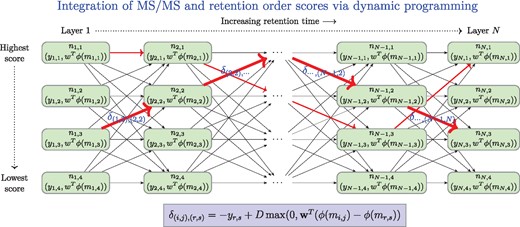
The scheme of the dynamic programming applied to find a set of identifications that maximize the combined score from IOKR and RankSVM for a set of (MS/MS, retention time) measurements. The layers correspond to candidate sets of molecules for a given MS/MS observed at given retention time. In each layer the candidate molecules are ordered by decreasing IOKR score, $y_{i,j}$⁠. The weight ${\delta }_{i,j,r,s}$ of the edge going from the node $n_{i,j}$ to $n_{r,s}$ is defined by the negative score of IOKR assigned to $n_{r,s}$⁠, and the score difference provided by the Rank SVM, i.e. ${\delta }_{i,j,r,s}=-y_{r,s}+D\max (0,w^T(\phi (m_{i,j})-\phi (m_{r,s})))$⁠. Some possible paths are shown by red arrows, potential optimum, the shortest path is denoted by the thick red arrows

Given the graph G, a path though the graph connects the layers $1,\dots ,N$ by picking one candidate structure for each measured MS/MS spectrum, and thus defines a sequence of molecular structures, taken as the identifications of the molecules generating the measurement data. Given a predefined weight for each edge, our dynamic programming algorithm efficiently finds a optimal path (one with smallest weight) among all possible paths connecting the nodes in the first layer to the nodes in the last layer.

Below, we define a edge weight function that combines the MS/MS based scores for candidate molecules from IOKR and the retention order scores from RankSVM in such a way that the dynamic programming solution jointly optimizes the total of MS/MS based scores and the retention order scores for all MS/MS measurements in the experiment and outputs an optimal sequence of candidate molecular structures, listed in their retention order.

In the construction of the graph G, the nodes are denoted by $n_{i,j}$ where $i=1,\dots ,N$ shows the layer containing the node and $j=1,\dots ,n_i$ gives the score related position within the column. Each node has the IOKR score denoted by $y_{i,j}$⁠. Two nodes are connected by a directed edge between two consecutive layers, thus there is an edge between any two nodes $n_{i,j}$ and $n_{r,s}$ if $r=i+1$⁠. To each edge a weight ${\text{δ}}_{(i,j),(r,s)}$ is assigned, and it is equal to

$${\text{δ}}_{(i,j),(r,s)}=-\underset{\text{IOKR score}}{\underbrace{y_{r,s}}}+\hspace{0.17em}D\underset{\text{penalty on order conflict}}{\underbrace{\max (0,w^T(\phi (m_{i,j})-\phi (m_{r,s}))}},$$

where w is provided by the RankSVM, and $\phi (m_{i,j})$ is the feature vector of the candidate molecule $m_{i,j}$ associated with kernel $k_m$⁠. The $\max (0,.)$ means that only the rank differences contradicting the order based on the retention time, as penalties, are considered in the edge weights. The constant D balances between the score and penalty term. We set the penalty term to zero, if the observed retention times of layer i and r are equal. The length of a path is defined by summing up the weight of the edges covered by that path. The main concepts of the optimization model are presented in Figure 3. The red arrows indicate two possible paths, corresponding to two sequences of candidate structures.

The dynamic programming algorithm (Table 1) goes through the graph sequentially from first layer to last layer. In each layer, for each node, the smallest weight path from the first layer to that node is stored along with the weight of the path. At the last layer, the optimal path is retrieved by finding the node with minimum weight path leading to it. The time complexity of the algorithm is $O(N{K}^2)$ where N is the number of layers and $K={\max }_{i=1}^N(n_i)$ is the maximum size of a layer.

Table 1.

Dynamic programming algorithm for finding the smallest weight path through a layered directed graph G

Algorithm 1 Dynamic programming to find the smallest weight path.
Input: Graph G with edge weights  δ
Output: Optimal node sequence from each layer $(j_1,j_2,\dots ,j_N)$
## Initialize the shortest path length, and parent node at each node ## First layer
Forj = 1 to n1
${\text{λ}}_{1,j}=-y_{1,j}$ # shortest path
$p_{1,j}=-1$ # parent node
## Other layers
Fori = 2 to N
Forj = 1 to ni
${\text{λ}}_{i,j}=\infty$
$p_{i,j}=-1$
## Roll out the dynamic programming updates
Fori = 1 to N – 1
Forj = 1 to ni
Fors = 1 to ni+1
If${\text{λ}}_{i+1,s}>{\text{λ}}_{i,j}+{\text{δ}}_{(i,j),(i+1,s)}$
${\text{λ}}_{i+1,s}={\text{λ}}_{i,j}+{\text{δ}}_{(i,j),(i+1,s)}$
$p_{i+1,s}=i$
## Roll back the path from the last layer to the first one
$j_N=\arg {\min }_j{\text{λ}}_{N_j}$ # End node of the optimum path
Path = [jN]
$\mathit{\text{Parent}}=p_{N,j_N}$
Fori = N – 1 to 1 step – 1
Path $\mathit{\text{=[Parent]+Path}}$
$\mathit{\text{Parent}}=p_{i,\mathit{\text{Parent}}}$

3 Results

In this section, we describe the datasets and protocols we use for the evaluation of the retention order prediction and metabolite identification. We present the results of our experiments and start with the analysis of the performance difference between binary and counting molecular fingerprints (Section 2.2.3) for the retention order prediction using RankSVM (Section 2.2.1). Subsequently we compare the RankSVM with the SVR (Section 2.2.2) in terms of order prediction performance. We close this section by an experiment using retention order prediction as additional source of information for the metabolite identification (Sections 2.3.1 and 2.3.2).

3.1 Retention order prediction

In this section, we evaluate the retention order prediction performance using RankSVM and SVR.

3.1.1 Dataset

We evaluate and compare our approach on five datasets extracted from the publicly available retention time database provided by Stanstrup et al. (2015). We used their R-package PredRetR to download the data and only considered measurements added before July 2015. The datasets contain retention time measurements from different reversed-phase chromatographic systems. Table 2 contains information about these datasets. The set S contains all those systems (Section 2.2.1). For compounds with multiple retention time measurements reported within one dataset we keep only the lowest retention time and remove the molecule completely when the lowest and the largest retention time differs by more than 5%. Furthermore, for each system we remove molecules with very small retention times from the dataset to avoid molecules that are not interacting with this chromatographic system. After the pre-processing the dataset contains 1098 retention time measurements of 946 unique molecular structures. We represent the molecular structure using MACCS fingerprints, which we calculate using the rcdk (Guha, 2007) R-package given the InChI representation of the molecular structures. We extended the current version of the CDK library (Willighagen et al., 2017), that is the back-end of rcdk, to support counting MACCS fingerprints. The similarity between molecules is measured using the Tanimoto kernel for binary and the MinMax kernel for counting fingerprints (Section 2.2.3). We use the same kernels for the RankSVM and the SVR.

Table 2.

Summary of the retention time datasets used in our experiments

Dataset / System	Column	# of Measurements
Eawag_ XBridgeC18	XBridge C18 3.5u 2.1x50 mm	317
FEM_long	Waters ACQUITY UPLC HSS T3 C18	281
RIKEN	Waters ACQUITY UPLC BEH C18	181
UFZ_ Phenomenex	Kinetex Core-Shell C18 2.6 um, 3.0 x 100 mm, Phenomenex	192
LIFE_old	Waters ACQUITY UPLC BEH C18	127
Impact	Acclaim RSLC C18 2.2um, 2.1x100mm, Thermo	342

Notes: The number of molecules corresponds to the one after the pre-processing. The Impact dataset is only used for our metabolite identification experiment.

3.1.2 Evaluation protocol

The evaluation is performed using 10-fold cross-validation (10-CV) produced such that no molecular structure of the training set is within the test set. For the hyper-parameter estimation, e.g. C parameter of the RankSVM, we use a nested 10-CV on the training set. As performance measure we use the pairwise prediction accuracy, that is the fraction of correctly classified molecule pairs, in a particular system $s\in S$⁠:

$$\text{Pairwise accuracy}\equiv \frac{\left|\right\{(i,j)\in \mathcal{P}(s)|w^T{\phi }_i<w^T{\phi }_j\}|}{|\mathcal{P}(s)|},$$

where $w$ is the prediction model obtained by the RankSVM respectively the SVR. In the following, we call the system s that we use the access the pairwise prediction accuracy as target system. We average the pairwise prediction accuracy over 10 repetitions of 10-CV.

3.1.3 Accuracy of binary versus counting fingerprints

We train RankSVM separately for each target s using only the target systems training preferences $\mathcal{P}(s)$⁠. The results in Table 3 show that the counting fingerprints outperform the binary ones. This indicates that the knowledge of the abundance of certain molecular sub-structures carries additional information, over binary fingerprints, about the retention behavior of a molecule. For the subsequent experiments, we therefore use the counting fingerprints with the MinMax kernel.

Table 3.

Pairwise prediction accuracy (⁠$\pm 2\text{σ}$⁠) for the different target systems (datasets) comparing binary and counting MACCS fingerprints

Target system s	Binary MACCS	Counting MACCS
Eawag_XBridgeC18	$0.796(\pm 0.015)$	$0.8\mathrm{4}4(\pm 0.0\mathrm{1}1)$
FEM_long	$0.882(\pm 0.016)$	$0.9\mathrm{0}5(\pm 0.0\mathrm{1}5)$
RIKEN	$0.826(\pm 0.024)$	$0.8\mathrm{4}8(\pm 0.0\mathrm{1}7)$
UFZ_Phenomenex	$0.790(\pm 0.027)$	$0.8\mathrm{0}2(\pm 0.0\mathrm{1}7)$
LIFE_old	$0.842(\pm 0.050)$	$0.8\mathrm{6}2(\pm 0.0\mathrm{3}5)$

Boldface denotes the method achieving the highest pairwise prediction accuracy. Note: Models were trained using $\mathcal{P}(s)$⁠.

3.1.4 Retention order prediction: RankSVM versus SVR

We compare the RankSVM and SVR performance in two experimental settings. In the first setting, the RankSVM or SVR model of one system s is trained using only the training preferences $\mathcal{P}(s)$ of this target system. In the second setting, a set $\mathcal{P}\setminus \mathcal{P}(s)$ [Equation (1)] of preferences originating from other chromatographic systems is used in addition to $\mathcal{P}(s)$ to train the model of the system s. This second experiment is motivated by the fact that large sets of retention times can be available, but those might be measured with different chromatographic systems. Then in both settings we vary the percentage of target system retention time measurements used for training from 0% (10% in the first setting) to 100%. This simulates the application case, where no or only a few retention time measurements are available in the target system s.

Single system for training: In Table 4 first pair of columns, Single system, target data only, we show the pairwise prediction accuracy for the RankSVM and SVR when we train using only training data of the target system s. RankSVM and SVR perform almost equally good in retention order prediction when using only target system training data. In Figure 4 (dashed lines) we plot the pairwise prediction accuracy as a function of the percentage of target system data used for training. Adding more data improves the accuracy of the models. Also in this case, RankSVM and SVR have almost the same behavior.

Table 4.

Pairwise prediction accuracy (⁠$\pm 2\text{σ}$⁠) comparing the different prediction methods and experimental settings for each target systems s individually

	Single system, target data only		Multiple systems, no target data		Multiple systems, all data
Training pref. (% of target)	$\mathcal{P}(s)$ (⁠$100\%)$	$\mathcal{P}(s)$ (⁠$100\%)$	$\mathcal{P}\setminus \mathcal{P}(s)$ (⁠$0\%)$	$\mathcal{P}\setminus \mathcal{P}(s)$ (⁠$0\%)$	$\mathcal{P}$ (100%)	$\mathcal{P}$ (100%)
Target system s	RankSVM	SVR	RankSVM	SVR	RankSVM	SVR
Eawag_XBridgeC18	$0.844(\pm 0.011)$	$0.846(\pm 0.011)$	$0.776(\pm 0.012)$	$0.719(\pm 0.006)$	$0.8\mathrm{6}7(\pm 0.0\mathrm{1}1)$	$0.736(\pm 0.014)$
FEM_long	$0.905(\pm 0.015)$	$0.904(\pm 0.014)$	$0.864(\pm 0.010)$	$0.717(\pm 0.020)$	$0.9\mathrm{1}3(\pm 0.0\mathrm{0}9)$	$0.819(\pm 0.011)$
RIKEN	$0.848(\pm 0.017)$	$0.842(\pm 0.020)$	$0.852(\pm 0.010)$	$0.755(\pm 0.018)$	$0.8\mathrm{6}7(\pm 0.0\mathrm{1}2)$	$0.742(\pm 0.015)$
UFZ_Phenomenex	$0.802(\pm 0.017)$	$0.796(\pm 0.023)$	$0.836(\pm 0.013)$	$0.702(\pm 0.021)$	$0.8\mathrm{4}8(\pm 0.0\mathrm{0}9)$	$0.731(\pm 0.017)$
LIFE_old	$0.862(\pm 0.035)$	$0.860(\pm 0.028)$	$0.873(\pm 0.019)$	$0.748(\pm 0.029)$	$0.8\mathrm{9}9(\pm 0.0\mathrm{1}8)$	$0.704(\pm 0.046)$

Boldface denotes the method achieving the highest pairwise prediction accuracy.

Fig. 4.

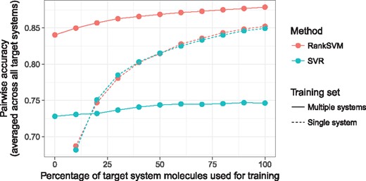
Pairwise prediction accuracy as a function of percentage of the target systems data used for training. Here we average the curves over the different target systems. The dashed lines correspond to the setting, where we use only a single system to train the order prediction. This curve starts at 10% as less data would be not sufficient for the learning. The solid lines show the behavior in the case where multiple systems are used for training

Multiple systems for training: In Table 4, the last two pairs of columns summarize the pairwise prediction accuracies when we train the RankSVM and SVR using the data from other chromatographic systems than the target system (preference set $\text{P∖P}(s)$⁠) in addition or in place of the data from the target system itself (preference set $\mathcal{P}(s)$⁠). In the columns Multiple systems, no target data, for the RankSVM it can be seen, that for three out of five target systems the prediction performance when we train only with the retention time information of the other chromatographic systems (preference set $\mathcal{P}\setminus \mathcal{P}(s)$⁠) performs at least as good as training with the single target system. When we include all the target system information (columns Multiple systems, all data) into the learning (preference set $\mathcal{P}$⁠) then we always outperform the baseline using a single system. That means that we can use the retention time information from different chromatographic systems to train a model for a single target system, that outperforms the one training only on the target system. The results furthermore show that the SVR do not benefit from retention time data that comes from different chromatographic systems. Training a model on the single target system always outperforms the model with more data. An explanation for this behavior is that the retention times across different chromatographic systems can be very different, e.g. the same molecule can have different retention times in different systems. In Figure 4, we plot the pairwise prediction accuracy as a function of the percentage of target system data used for training. For the RankSVM model, we observe that adding more data from the target system can improve the model. For the SVR the performance improvement is smaller and as the models starts of at low accuracy it cannot outperform the SVR model trained on the single target system.

3.2 Metabolite identification

In this section, we describe the evaluation of our proposed method to combine MS/MS based scores and predicted retention orders for metabolite identification. For that we use LC-MS/MS data from MassBank arising from a single system, where a set of MS/MS spectra and the corresponding retention times are given, to construct an artificial dataset that could arise in a single LC-MS/MS run. The task is to identify the correct molecular structures for each MS/MS spectrum by utilizing the observed retention times of the unknown compounds.

3.2.1 Dataset

We extracted retention times for molecules measured with the same reversed-phase chromatographic system (Table 2, Impact) from Massbank (Horai et al., 2010). In the following, we will refer to this dataset as Impact. All measurements are provided by the Department of Chemistry of the University of Athens (record prefix: AU). After the pre-processing (Section 3.1.1) retention time measurements of 342 different molecular structures remained. For each compound, we searched for a corresponding MS/MS spectrum in the GNPS (Wang et al., 2016) spectra database. This resulted in MS/MS spectra for 120 compounds. For each compound m_i in this set, we obtained a set of molecular candidates ${\mathcal{M}}_i=\left\{m_{i,j}\right\}$ by querying the molecules in the structure database Pubchem (Kim et al., 2015) with the same molecule formula as m_i. The resulting dataset is used in our experiments as a model of data that can arise in a LC-MS/MS experiment, however, equipped with ground truth identifications due to the above construction. To calculate the IOKR score for each candidate $m_{i,j}$ as described in Section 2.3.1, we use the same MS/MS spectra kernels and molecular fingerprints as Dührkop et al. (2015). As the output kernel k_m we use a Gaussian kernel in which distances are derived from the Tanimoto kernel (Section 2.2.3): $k_m(m_i,m_j)=\exp \left(-\text{γ}\left|\right|{\text{ψ}}_i-{\text{ψ}}_j|{|}^2\right)$⁠, where ψ_i and ψ_j are the feature vectors associated with the Tanimoto kernel, and $\text{γ}>0$ is a scaling parameter. The 222 compounds without MS/MS spectra, are used as training data for the RankSVM.

3.2.2 Evaluation protocol

The metabolite identification performance is measured by the percentage of correct molecular structures along the shortest path found by dynamic programming approach presented in Section 2.3.2. In the following, we refer to this performance measure as identification accuracy. We compare our approach to integrate the MS/MS based (IOKR) scores and the predicted retention orders (D > 0) with the baseline performance, when only the IOKR scores are used (D = 0) for the identification. We randomly sample 1000 times 80 MS/MS spectra and calculate the average identification accuracy separately for different values of D.

3.2.3 Integrating IOKR scores and predicted orders

The target system in this experiment refers to Impact, as the system that provides the retention times for the MS/MS spectra. We train three different RankSVM models, the order predictor, using MACCS counting fingerprints and three different retention time training sets:

• Target, $\mathcal{P}(s_{\text{Impact}})$⁠: Retention times for 222 compounds measured with the Impact system. None of these compounds is part of the LS-MS/MS dataset.

• Others, $\mathcal{P}$⁠: Retention times for 946 unique compounds measured with different chromatographic systems (Sections 3.1.1).

• Others & target, $\mathcal{P}\cup \mathcal{P}(s_{\text{Impact}})$⁠: Retention time measurements from the target and other chromatographic systems.

Figure 5 shows the average identification accuracy from 1000 random samples of 80 MS/MS spectra for different values of D. The baseline performance when D = 0, i.e. only the IOKR scores are used, is 22.7% (shown as black solid line). When the RankSVM is trained using retention times from the target system and other chromatographic systems (Others & target) the metabolite identification accuracy can be improved up to 24.8% at D = 0.0075. This is an significant improvement over the baseline (P-value smaller $2.2{\text{e}}^{-16}$ using the one-sample t-test). With 23.9% at D = 0.01 the performance improvement is smaller when only retention times from other chromatographic systems (Others) are used, but still significant (P-value smaller $2.2{\text{e}}^{-16}$⁠). Using only target system retention times is not sufficient to improve the metabolite identification performance. The overall trend in the results is that the larger the training set for the RankSVM the larger improvement in metabolite identification accuracy. This observation is consistent with the results form the experiments evaluating the pairwise prediction performance of the RankSVM for different training sets (Section 3.1.4). The more retention time information is used to train the RankSVM, the more accurate the pairwise orders are predicted.

Fig. 5.

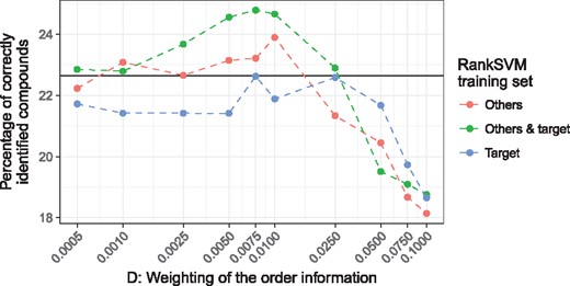
Average percentage of correctly identified molecular structures for different values of D. The baseline accuracy, when only the MS/MS based IOKR scores are used (D = 0) is shown as black solid line. We plot the accuracy for three different RankSVM training sets: Target, retention time data from target system, Others, retention time data only from other systems, Others & target, both previous sets together

4 Discussion

In this paper, we have put forward a new framework for predicting the retention order of molecules in liquid chromatography, and the integration of the retention order predictions to tandem MS based metabolite identification.

The methodology is based on ranking support vector machine (RankSVM) that uses molecular fingerprints of two molecules as input and the retention order as output. For input description, we found that so called counting fingerprints provide more accurate results than the more standard binary fingerprints. It thus seems that not only the presence of certain chemical groups but also their counts is important for the retention behaviour in LC.

We explored different settings for training retention time and retention order predictors. In particular, we found out that the RankSVM model is able to use retention order data from other chromatographic systems than the current target system to arrive at more accurate predictions. The support vector regression (SVR) method for predicting retention times, on the other hand, was limited in this capacity and required a much larger library of measurements conducted with the target system before the accuracy reached a reasonable level, after which point the data form the other systems provided no benefit. On contrast, the RankSVM model proved to benefit from the other systems without similar threshold point.

Furthermore, we proposed a method for integrating the retention order predictions to MS/MS based metabolite identification model IOKR. The method constructs a directed graph with edges linking molecules in the candidate lists of MS/MS spectra measured at adjacent retention times and assigns the IOKR scores as node weights, the retention order scores as edge weights and searcher for shortest path across this graph to find the highest scoring combination of metabolites. This approach was shown to have the capability to improve the number of correctly identified metabolites.

Acknowledgement

The authors would like to thank Emma Schymanski, Kris Morreel and Steffen Neumann for providing retention time datasets as well as fruitful discussions.

Funding

This work was supported by Academy of Finland [268874/MIDAS, 310107/MACOME]; and the Aalto Science-IT infrastructure.

Conflict of Interest: none declared.