A Boolean network inference from time-series gene expression data using a genetic algorithm

Abstract

Motivation

Inferring a gene regulatory network from time-series gene expression data is a fundamental problem in systems biology, and many methods have been proposed. However, most of them were not efficient in inferring regulatory relations involved by a large number of genes because they limited the number of regulatory genes or computed an approximated reliability of multivariate relations. Therefore, an improved method is needed to efficiently search more generalized and scalable regulatory relations.

Results

In this study, we propose a genetic algorithm-based Boolean network inference (GABNI) method which can search an optimal Boolean regulatory function of a large number of regulatory genes. For an efficient search, it solves the problem in two stages. GABNI first exploits an existing method, a mutual information-based Boolean network inference (MIBNI), because it can quickly find an optimal solution in a small-scale inference problem. When MIBNI fails to find an optimal solution, a genetic algorithm (GA) is applied to search an optimal set of regulatory genes in a wider solution space. In particular, we modified a typical GA framework to efficiently reduce a search space. We compared GABNI with four well-known inference methods through extensive simulations on both the artificial and the real gene expression datasets. Our results demonstrated that GABNI significantly outperformed them in both structural and dynamics accuracies.

Conclusion

The proposed method is an efficient and scalable tool to infer a Boolean network from time-series gene expression data.

Supplementary information

Supplementary data are available at Bioinformatics online.

1 Introduction

A gene regulatory network (GRN) is represented by a directed graph consisting of sets of nodes and directed edges, which represent genes/proteins and regulatory interactions among them, respectively. It is a fundamental problem in systems biology to infer a GRN from gene expression data as accurately as possible, because it helps us to understand complex biological processes through network-level analyses. As more time-series gene expression data is available due to recent advances in high-throughput microarray technology and RNA-Seq, a number of inference approaches have been developed using a variety of computational models such as a Boolean network (Kauffman, 1969), a Bayesian network (Imoto et al., 2002) and a differential equation model (Chen et al., 1999). Among them, a Boolean network where a state of a gene is represented by a Boolean value, 1 (ON) or 0 (OFF), and a regulatory interaction is represented by a Boolean function, is most efficient to represent a very large-scale network due to the simplest representation. However, most previous Boolean network inference methods still have a limitation in scalable representation of regulatory interactions. For example, the feasible number of regulatory genes was limited to only one to three in the well-known methods such as the reverse engineering algorithm (REVEAL) (Liang et al., 1998), Best-Fit (Lähdesmäki et al., 2003) and Bayesian inference approach for a Boolean network (BIBN) (Han et al., 2014). In addition, some other methods in the literature (Haider and Pal, 2012) are applicable only when some priori knowledge such as connectivity of regulator genes and state transition pairs are available.

To resolve the scalability problem, the mutual information (MI) was considered to efficiently identify the regulatory relations. For example, the relevance networks (RN) (Butte and Kohane, 2000) inferred a large number of regulatory genes by computing the pairwise MI values and discarding the genes with the lowest MI values, and the context likelihood of relatedness (CLR) (Faith et al., 2007) extended the relevance network using an adaptive background correction step. The algorithm for the reconstruction of accurate cellular networks (ARACNE) (Margolin et al., 2006) is another MI-based method which determines a significant dependency among genes using an inequality to filter out the weakest connections from every gene triplets. Despite a successful performance in each study, they cannot represent a real multivariate regulatory function because they examined only pairwise relations. In this regard, the mutual information-based Boolean network inference (MIBNI) (Barman and Kwon, 2017) to compute an approximated multivariate MI value was proposed in our previous study. Although it showed a better performance than the existing methods, there is a room for improvement because MIBNI was still a greedy algorithm based on the approximation metric. Alternatively, several ensemble methods to provide a set of solutions instead of a single solution were proposed by formulating a feature selection problem. For example, the gene network inference with ensemble of trees (GENIE3) (Irrthum et al., 2010) selects a set of features for random forests or extra trees learning models. Another method is the trustful inference of gene regulation using stability selection (TIGRESS) (Haury et al., 2012) which conducts a feature selection using the least angle regression integrated with a stability selection. Although both methods showed interesting performances, they eventually ranked linear relations of pairs of regulator and target genes. Considering that nonlinear regulatory relations are ubiquitously found in real biological networks, a method which can infer more generalized regulatory relations is required. To this end, we propose a novel genetic algorithm-based Boolean network inference (GABNI) method. Basically, it exploits MIBNI in the first stage to utilize the excellent performance in identifying regulatory rules of a small size. In case that MIBNI fails to find optimal solutions, a genetic algorithm is applied to search an optimal set of regulatory genes in a relatively huge problem space. GAs run for every target gene and all results are integrated into a final Boolean network. We validated the performance of GABNI with both the artificial and the real gene expression datasets through comparisons with four existing methods, MIBNI, ARACNE, GENIE3 and TIGRESS. Our method outperformed them in terms of both structural and dynamics accuracies, and this suggests that GABNI is a state of the art in Boolean network inference from a time-series gene expression dataset.

2 Materials and methods

2.1 A Boolean network model

In this study, we employed a Boolean network model to investigate the complex dynamics of gene regulatory network. A Boolean network (Kauffman, 1969) is represented by a directed graph G(V, A) where $V=\{v_1,v_2,\dots ,v_N\}$ is a set of nodes and $A=\{(v_i,v_j)\}\subseteq V\times V$ is a set of interactions. The value of a node $v_i\in V$ at time-step t + 1 denoted by $v_i(t+1)$ is updated by a Boolean function $f_i:{\{0,1\}}^{k_i}\to \{0,1\}$ of the values of k_i regulatory genes $v_{i_1},v_{i_2},\dots ,v_{i_{k_i}}$at time t. Hence, the update scheme of v_i can be written as

$$v_i(t+1)=f_i(v_{i_1}(t),v_{i_2}(t),\dots ,v_{i_{k_i}}(t)).$$

We note that a total of $2^{2k_i}$ Boolean functions are possible for f_i, and the update time lag is one.

2.2 The Boolean network inference problem

The Boolean network inference problem is a problem to infer not only a set of interactions but also a set of update functions from a time-series gene expression data. The inference performance can be assessed by comparing the trajectory generated by the inferred network and the observed time-series gene expression. Let $v\prime (t)$ the estimated value of gene v at time t in the inferred Boolean network. We define the gene-wise dynamics consistency $C(v,v\prime )$ as the similarity between the Boolean trajectories of the observed gene expression v(t) and the estimated gene expression $v\prime (t)$⁠, as follows:

$$C(v,v\prime )=\frac{{\sum }_{t=2}^{T}I(v(t)=v\prime (t))}{T-1},$$

(1)

where T is the total number of time-steps, and $I(·)$ is an indicator function that returns 1 if the condition is true, otherwise 0. In addition, the comparison starts at t = 2 by the assumed update time lag in this study. We finally define the dynamics accuracy of an inferred network as the average of gene-wise dynamics over all genes as follows:

$$\text{DynamicsAccuracy}=\frac{{\sum }_{i=1}^{N}C(v_i,v{\prime }_i)}{N}.$$

2.3 Structural performance metrics

When the structure of a gold standard or correct network is known, we can further evaluate the inference performance with respect to the network structure. To this end, we used three measures, precision, recall and structural accuracy. Precision is the ratio of correctly inferred connections over the total number of predictions as follows:

$$\text{Precision}=\frac{TP}{TP+FP},$$

where TP (true positive) and FP (false positive) denote the numbers of correctly and incorrectly predicted connections, respectively. Recall is the ratio of true predicted connections over the total number of actual connections:

$$\text{Recall}=\frac{TP}{TP+FN},$$

where FN (false negative) means the number of non-inferred connections in G(V, A). Structural accuracy is the ratio of correct predictions out of all predictions as follows:

$$\text{Structural}\hspace{0.17em}\text{Accuracy}=\frac{TP+TN}{TP+FP+FN+TN},$$

where TN (true negative) is the number of correct negative predictions.

2.4 MIBNI method

In this study, we propose a new inference algorithm which utilizes the strength of MIBNI (see Barman and Kwon, 2017 for details), which is a mutual information-based Boolean network inference algorithm with a limited update scheme. It has two subroutines, MIFS and SWAP. The MIFS subroutine returns an initial set of regulatory genes $S_v\subseteq V$ for each target gene v by computing an approximated multivariate mutual information. Then, the SWAP subroutine is applied to improve the dynamics accuracy by swapping between a selected regulatory genes S_v and the set of unselected genes $V\setminus S_v$⁠. It is repeated until there is no improvement in terms of the gene-wise dynamics consistency. MIBNI showed a superior performance for a relatively small number of regulatory genes with a small running time in the previous study. However, it has a limitation that only conjunction or disjunction Boolean functions are considered for representation of regulatory relations.

3 Our proposed method

In this paper, we propose a novel method called GABNI for a Boolean network inference from gene expression data. Figure 1 illustrates the overall framework of it. A time-series gene expression dataset is given as an input and it is converted into a binarized gene expression dataset using a K-means discretization method (MacQueen et al., 1967). It divides all expression values of each gene into two clusters, marked by 1(ON) and 0(OFF), which denote higher and lower than the average expression level, respectively. Given a target gene, MIBNI is first applied to infer an optimal update rule with a limited function scheme. If it fails to find the optimal rule (i.e. the gene-wise dynamics consistency is not equivalent to 1.0), our genetic algorithm is applied. The reason for this hybrid approach is that MIBNI can rapidly find an optimal solution in the case of a small-size problem as shown in the previous study (Barman and Kwon, 2017). We repeat this process for all target genes and eventually construct a final inferred network by integrating all found regulatory rules. In the following subsections, we describe the proposed GA in detail.

Fig. 1.

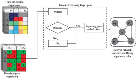
Overall framework of GABNI. A time-series gene expression data is converted into binary values. If MIBNI finds an optimal regulatory rule, it is included in the final inferred network. Otherwise, GA is applied to find a better solution. This process is executed for every target gene. All inference results are collected to construct the final inferred Boolean network

3.1 Our GA

The GA framework we used in this paper is shown in Figure 2. A chromosome represents a set of regulatory genes for a given target gene. The GA starts by randomly initializing the population P which is a set of chromosomes. Two parent chromosomes p₁ and p₂ are chosen by a roulette wheel selection, and then generate two offspring chromosomes x₁ and x₂ by a crossover operator. Each offspring can be mutated with a small probability. If the offspring is better than the parent, the former replaces the latter in the next generation. This process continues until a stopping criterion is met.

Fig. 2.

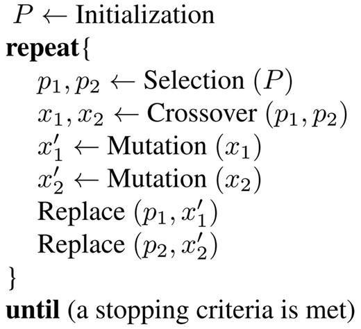
The framework of our GA

3.1.1 Chromosome representation

In our problem, the GA is used to select an optimal set of regulatory genes. Given a target gene $v\in V=\{v_1,\dots ,v_N\}$⁠, a chromosome is represented by a binary vector of length N where i-th element value (either 1 or 0) means that v_i is included or not in the set of regulatory genes. To reduce the search space of the GA, we set two constraints about the feasible solutions, the maximum number of regulatory genes and the minimum mutual information with the target gene. In other words, the GA does not consider a chromosome representing too many regulatory genes by the first constraint. In addition, the second constraint excludes the genes which are mostly uncorrelated to the target gene from the candidate solutions.

3.1.2 Fitness evaluation

A chromosome in the GA represents only the set of selected regulatory genes. Thus, we need to specify a regulatory rule from the chromosome to evaluate its fitness. Let v a target gene and $u_1,u_2,\dots ,u_k$ a set of selected regulatory genes in a chromosome. For simplicity, we denote a vector of values of genes $u_1(t),u_2(t),\dots ,u_k(t)$ by $\mathbf{u}(t)$⁠. To specify the regulatory rule of the chromosome, we estimate the value of v at time t + 1, denoted by $v\prime (t+1)$⁠, given a condition $\mathbf{u}(t)=\mathbf{b}$ for every bit string $\mathbf{b}=b_1{b}_2\cdots b_k\in {\{0,1\}}^k$⁠. Let $\Sigma =\{t\in \{1,\dots ,T-1\left\}\right|\mathbf{u}(t)=\mathbf{b}\}$⁠. If $|\Sigma |=0$ in the binary gene expression dataset, we set $v\prime (t+1)=\ast$ (don’t care symbol). Otherwise, we specify it as $v\prime (t+1)=\underset{b\in \{0,1\}\hspace{0.17em}}{\arg \max }\mathrm{Pr}(v(t+1)=b|\mathbf{u}(t)=\mathbf{b})$ in the binary gene expression dataset. In this way, we can specify $v\prime (t+1)$ for all bit strings $\mathbf{b}=b_1{b}_2\cdots b_k$ and eventually compute the gene-wise dynamics consistency [see Equation (1) in Section 2]. We note that $v\prime (t+1)$ is the optimal estimation given a set of input variables, $u_1,u_2,\dots ,$ and $u_k,$ with respect to the binary gene expression dataset. Figure 3 shows an example of the binary gene expression dataset with 10 genes measured for five time-steps. Given a target gene v₃, the example chromosome 0101000010 means that v₂, v₄ and v₉ are selected for regulatory genes. In the case of $v_2(t)v_4(t)v_9(t)=001$ (or 111), $v{\prime }_3(t+1)$ is specified to 0 (resp. 1) because $v{\prime }_3(t+1)$ is more likely to turn off (resp. on) in the binary gene expression dataset. On the other hand, $v{\prime }_3(t+1)$ is not specified in the case of $v_2(t)v_4(t)v_9(t)=100$ because there is a tie (we denote it by $“-”$ symbol). In addition, $v{\prime }_3(t+1)$ is not determined in the rest cases because the bit string was not observed in the dataset (we denote it by $“\ast ”$ symbol). We note that these non-deterministic cases marked by either $“\ast ”$ or $“-”$ symbol do not affect the gene-wise dynamics consistency. Next, we define the fitness function of a chromosome using the gene-wise dynamics consistency as follows:

$$Fitness=\frac{1}{(1-C(v,v\prime ))·\gamma +k}$$

where γ is a weight factor and k is the number of regulatory genes chosen by a chromosome. In other words, the fitness of a chromosome is larger as $C(v,v\prime )$ is larger and k is smaller. We set γ such that $(1-C(v,v\prime ))·\gamma \gg k$⁠, which implies that $C(v,v\prime )$ and k are considered as the primary and secondary factors for the fitness function, respectively.

Fig. 3.

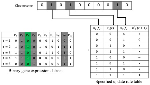
An example of specifying the update rule from a chromosome. Assume that the binary gene expressions of 10 genes are measured over five time-steps. Let v₃ a target gene and consider a chromosome 0101000010 where v₂, v₄ and v₉ are selected as a set of regulatory genes. The best estimated value of the target gene, $v_3^{\prime }(t+1)$⁠, is determined for every $2_{}^3$ bit strings of regulatory genes from the binary gene expression dataset. The symbol ‘*’ means that the given bit string was not observed in the gene expression dataset. The symbol ‘–’ means that the best estimation value is a tie between 0 and 1. We note that these unspecified symbols do not affect the gene-wise dynamics consistency

3.1.3 Selection, crossover and mutation

Our GA chooses two parent solutions among the population using a variant roulette wheel selection. The selection probability of a chromosome is proportional to the adjusted fitness defined as follows:

$$Adjusted\hspace{0.17em}Fitness=\alpha \times Fitness+\beta$$

where $\alpha =\frac{H}{FMAX-FMIN}$ and $\beta =1-\alpha ·FMIN$⁠. Herein, $FMAX$ (and $FMIN$⁠) means the maximum (resp. minimum) fitness value in the population, and H is an adjustment parameter. We note that this linear adjustment assigns the selection probability of the best chromosome to H times of that of the worst chromosome in the population. It helps the GA to avoid a premature convergence.

Once two parent chromosomes are selected, a crossover is applied to produce two offspring chromosomes as shown in Figure 4. Unlike most general crossovers such as multi-point crossover, we devised a new crossover which can more properly inherit the membership information of genes in parents. If a binary gene value is common in both parents, it is copied to an offspring (the white or gray gene in Fig. 4). Otherwise, a value selected between two parents uniformly at random is copied to an offspring (the yellow or blue gene in Fig. 4). Each offspring chromosome can be modified by a bitwise uniform mutation operator, which flips every bit value with a small probability.

Fig. 4.

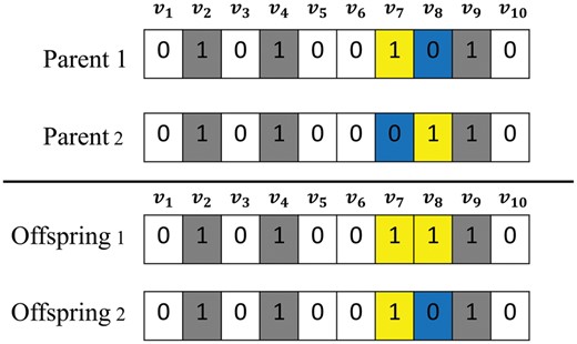
The crossover operator used in this study. Parent 1 and 2 include $\{v_2,v_4,v_7,{\mathrm{v}}_9\}$ and $\{v_2,v_4,v_8,{\mathrm{v}}_9\}$ for regulatory gene sets, respectively. A bit value common to both parents is copied to an offspring (white or gray color). Otherwise, a bit value between two parents is selected at uniform random (yellow or blue color)

3.1.4 Replacement and stopping criterion

If the offspring is superior to the parent, the former replaces the latter in the population at the next generation. The GA repeats the evolution of new solutions and stops after a fixed number of generations.

3.2 Identification of an interaction type

Most previous inference methods focus on the inference of interactions between a target and a regulator gene. However, it is also important to identify the interaction type, i.e. a positive (activating) or negative (inhibitory) interaction. To this end, GABNI infers the interaction type by examining the binary expression values of a target gene and a regulatory gene in the binary gene expression data. Let v and u be a target and a regulatory gene, respectively, in the inference result by GABNI. In addition, let $C_{ij}=\left|\right\{t\in \{1,\dots ,T-1\}|v(t+1)=i \text{and} u(t)=j\}|$ in the binary gene expression dataset. If $C_{00}+C_{11}\ge C_{01}+C_{10}$⁠, u activates v. Otherwise, u inhibits v.

4 Results

To validate our approach, we tested GABNI with two kinds of datasets, the artificial and the real time-series gene expression datasets, and showed the results in Sections 4.1 and 4.2, respectively. Table 1 shows the parameter values of the GA we specified in this work.

Table 1.

GA parameter values in this study

Parameters	Value
Population size	N + 10
Maximum number of regulatory genes	$0.6·N$
Minimum mutual information with the target gene	0.05
γ in fitness function	28
H in adjusted fitness	3
Number of GA iterations	1000
Mutation probability	0.01

4.1 Performance on the artificial gene expression dataset

We used two kinds of random network generation models to create artificial gene expression datasets, the Barabasi-Albert (BA) model (Barabasi and Albert, 1999) and the GeneNetWeaver (GNW) tool-based model (Schaffter et al., 2011). In the BA model, we first generated 10 random networks with different network sizes (⁠$\left|V\right|=10,20,\dots ,100$ and $\left|A\right|=2·\left|V\right|$⁠) using a preferential attachment mechanism (see Supplementary Fig. S1 for the pseudo-code). Then we randomized a set of update functions and generated a time-series trajectory starting with a random initial state. For a more stable test, we repeated it 30 times. As a result, we tested GABNI over a total of 300 different datasets based on the BA model. In the GNW model, the tool generates random network structures by referring to a real E. coli or S. cerevisiae regulatory network. For each $\left|V\right|=10,20,\dots ,100$⁠, we generated 30 networks with different numbers of interactions (⁠$\left|A\right|\in [27,204]$⁠; see Supplementary Table S1). The generated continuous expression values were converted into Boolean values using K-means algorithm. The maximum time-step (T) was set to $\left|V\right|+10$ for both BA and GNW models. We compared GABNI with four previous methods MIBNI, ARACNE, GENIE3 and TIGRESS.

4.1.1 Structural accuracy comparison

As explained before, we tested five inference methods over two sets of 300 random gene expression datasets generated by BA and GNW models. The results with respect to the structural inference accuracy are shown in Figure 5 (BA model) and Supplementary Figures S2–S4 (GNW model). For more detailed analysis, we classified the target genes into nine classes according to the incoming links (D) which was ranged from 1 to 9. As shown in Figure 5, the structural performance of all methods decreases as the incoming links increases. This is because the number of incoming links eventually represents the degree of difficulty of an inference problem. GABNI and MIBNI showed perfect performances in the case of D = 1. This is not surprising because the GA operates only when MIBNI fails to find an optimal solution. On the other hand, GABNI more significantly outperforms other methods as D increases. This implies that our GA dramatically improved the structural inference performance over the other methods. These results are consistently observed irrespective of a specific network size (see Supplementary Figs S5–S7 for details), and in GNW random networks (See Supplementary Figs S2–S4 for details).

Fig. 5.

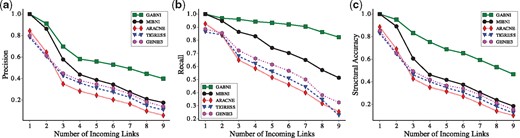
Comparison of precision, recall and structural accuracy between GABNI and other methods in BA random networks. Results of (a) precision, (b) recall and (c) structural accuracy, respectively. Ten random networks with different network sizes $\left|V\right|=10,20,\dots ,100$ were created and 30 random trajectories for each network were generated. A total of 16 500 nodes in those networks were classified into nine groups according to the number of incoming links. Y-axis values show the average precision, recall and structural accuracy values in each group. GABNI showed the best performance in terms of precision, recall and structural accuracy

4.1.2 Dynamics accuracy comparison

In this subsection, we analyzed the performance with respect to the dynamics accuracy in Figure 6 (BA model) and Supplementary Figure S8 (GNW model). As shown in Figure 6a, we computed the average dynamics accuracy against the network sizes, $\left|V\right|=10,20,\dots ,100$⁠. Interestingly, the dynamic accuracy of GABNI was 1.0 (perfect accuracy) for all network sizes whereas that of MIBNI, ARACNE, GENIE3 and TIGRESS methods decreased as the network size increased. This implies that our GA always found the optimal solutions in terms of the fitness value. We observed a consistent result in the case of GNW random networks (see Supplementary Fig. S8). We further examined the change of dynamics accuracy of the best solutions in GA against the number of generations (Fig. 6b). As expected, the dynamics accuracy of the best solution in GA gets lower as the number of incoming links is larger. However, it almost finds the optimal solution around 600 generations regardless of the number of incoming links. This implies that our GA is considerably robust against the degree of difficulty of the inference problem.

Fig. 6.

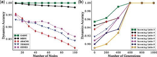
Dynamics accuracy analysis in BA random networks. (a) Comparison of dynamic accuracies between GABNI and other methods in BA random networks. Ten random networks with different network sizes $\left|V\right|=10,20,\dots ,100$ were created and 30 random trajectories for each network were generated. Therefore, each point means the average dynamics accuracy of a method over 30 datasets. (b) Change of dynamics accuracy against the number of generations in GA. BA random networks with $\left|V\right|=100$ were analysed. We classified the target genes according to the number of incoming links (D) and examined the change of the average dynamics accuracy of the best solutions for every 200 generation in GA

4.1.3 Computation time comparisons

The comparative result of the running time among GABNI, MIBNI, ARACNE, GENIE3 and TIGRESS over 300 BA random networks is shown in Figure 7. All simulations were executed on a PC with Intel Core i7 3.4 GHz CPU and 8GB memory using a single processor core. As shown in the figure, MIBNI was fastest whereas GABNI was slowest among them, because GA is a global optimization method to search a wide range of candidate solutions. This implies that our method finds a high-quality solution by sacrificing the search time. In addition, we note that the usage of MIBNI in the first stage of the GABNI framework is beneficial to not only the accuracy performance but also the running time.

Fig. 7.

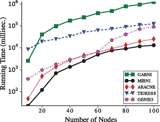
Comparison of the running time among the network inference methods. The Y-axis values represent the average log-scaled running time of GABNI, MIBNI, ARACNE, TIGRESS and GENIE3. MIBNI was fastest among them. On the other hand, GABNI was slowest because it searches a larger problem space. The time unit is measured in millisecond

4.2 Performance on the real gene expression dataset

4.2.1 Case study 1: DREAM challenge dataset

We applied GABNI to infer signaling networks from DREAM challenge datasets (Marbach et al., 2010; Prill et al., 2010; Stolovitzky et al., 2007). There are five datasets of two E. coli and three Yeast networks, and every gold standard network consists of 10 genes. In addition, they have 10, 15, 15, 22 and 25 interactions, respectively, and each dataset was measured over 21 time points. Tables 2 and 3 summarize the structural and the dynamics accuracies, respectively. Both accuracies of GABNI were significantly higher than those of the other methods in all datasets. In addition, GABNI greatly improved the performance of MIBNI in all datasets, which implies that our genetic search was efficient and robust.

Table 2.

Structural accuracies in DREAM3 challenge

Methods	E. coli 1	E. coli 2	Yeast 1	Yeast 2	Yeast 3
GABNI	0.9042	0.8762	0.9340	0.8252	0.8265
MIBNI	0.8437	0.7979	0.8315	0.7075	0.7102
ARACNE	0.7035	0.7800	0.7034	0.6247	0.5637
GENIE3	0.8144	0.7920	0.7567	0.6846	0.6296
TIGRESS	0.8063	0.7857	0.7319	0.6699	0.6017

Table 3.

Dynamics accuracies in DREAM3 challenge

Methods	E. coli 1	E. coli 2	Yeast 1	Yeast 2	Yeast 3
GABNI	1.0000	0.9800	0.9800	0.9700	1.0000
MIBNI	0.9400	0.9200	0.9200	0.9200	0.8900
ARACNE	0.8200	0.8900	0.8500	0.8800	0.7700
GENIE3	0.8800	0.9000	0.8900	0.9100	0.9000
TIGRESS	0.8500	0.9000	0.9000	0.9000	0.8600

4.2.2 Case study 2: Budding yeast cell cycle

In the second case study, we applied GABNI to infer a budding yeast cell cycle network consisting of $\left|V\right|=11$ nodes and $\left|A\right|=29$ interactions (Li et al., 2004; Fig. 8). In the previous study, a Boolean time-series gene expression dataset was given (see Supplementary Table S2). As shown in Figure 8b, our method correctly inferred 18 true connections out of 29 connections. On the other hand, MIBNI, ARACNE, GENIE3 and TIGRESS correctly identified 14, 11, 14 and 14 connections, respectively. Specifically, the structural accuracies of GABNI, MIBNI, ARACNE, GENIE3 and TIGRESS are 0.8843, 0.8240, 0.8125, 0.8080 and 0.8080, respectively. In addition, the dynamics accuracy of GABNI was 1.0 (perfect accuracy) whereas those of MIBNI, ARACNE, GENIE3 and TIGRESS were approximately 0.9600, 0.9600, 0.9800 and 0.9500, respectively (see Supplementary Fig. S9 for details). In other words, GABNI showed significantly better performance than the other methods in terms of both structural and dynamics accuracies. Furthermore, we examined the performance sensitivity against the noise effect. We flipped 5% and 10% binary gene expression values among the dataset and observed GABNI robustly outperformed the other methods (see Supplementary Table S3).

Fig. 8.

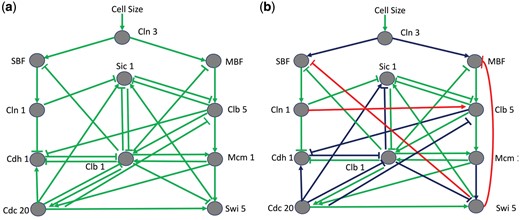
Application of GABNI to infer the budding yeast cell cycle network. (a) The gold standard of the budding yeast cell cycle network. It consists of 11 genes and 29 interactions. (b) Inference result by GABNI. The green, red and blue interactions denote true positive, false positive and false negative predictions, respectively. The inferred result shows 18 true positives, 3 false positives and 11 false negatives. The structural and dynamics accuracies were 0.8843 and 1.0 (perfect prediction), respectively

5 Conclusions and discussion

In this work, we proposed a novel Boolean network inference method from time series gene expression data using a genetic algorithm, called GABNI. Although many previous methods were suggested for network inference, they were not efficient in inferring a regulatory relation involving a large number of genes. In addition, some of them outputs only a set of regulatory genes without detailed specification of a regulatory rule. Our proposed method exploited an existing method, MIBNI, in the first stage because it can almost find an optimal solution for a relatively less complex problem even with a very short running time. If MIBNI fails to find an optimal solution due to the degree of complexity of an underlying regulatory function, our GA is applied. In particular, we modified a typical GA framework by suggesting the representation constraints and a sort of membership crossover for an efficient search. We validated our method through extensive comparisons with four other methods, MIBNI, ARACNE, GENIE3 and TIGRESS, over both the artificial and the real gene expression data. In particular, GABNI significantly outperformed the other methods for larger-scale inference problems in terms of both the structural and the dynamics accuracies. Although the running time of GABNI was largest, it is possible to reduce the running time by parallel implementation, which will be included in a future study.

Funding

This work was supported by the 2018 Research Fund of University of Ulsan.

Conflict of Interest: none declared.