Single cell network analysis with a mixture of Nested Effects Models

Abstract

Motivation

New technologies allow for the elaborate measurement of different traits of single cells under genetic perturbations. These interventional data promise to elucidate intra-cellular networks in unprecedented detail and further help to improve treatment of diseases like cancer. However, cell populations can be very heterogeneous.

Results

We developed a mixture of Nested Effects Models (M&NEM) for single-cell data to simultaneously identify different cellular subpopulations and their corresponding causal networks to explain the heterogeneity in a cell population. For inference, we assign each cell to a network with a certain probability and iteratively update the optimal networks and cell probabilities in an Expectation Maximization scheme. We validate our method in the controlled setting of a simulation study and apply it to three data sets of pooled CRISPR screens generated previously by two novel experimental techniques, namely Crop-Seq and Perturb-Seq.

Availability and implementation

The mixture Nested Effects Model (M&NEM) is available as the R-package mnem at https://github.com/cbg-ethz/mnem/.

Supplementary information

Supplementary data are available at Bioinformatics online.

1 Introduction

Understanding heterogeneous diseases like cancer on the molecular level is challenging, but also crucial for the development and improvement of therapies. Molecular intra-tumor heterogeneity is an important factor for cancer treatment (Prasetyanti and Medema, 2017; Sun and Yu, 2015). Treatment strategies often assume cancer to be homogeneous across cells. However, if different cell types are resistant to different drugs, the success of current treatment strategies is limited.

A key component of the molecular landscape are signaling pathways and how they are causally wired in healthy and diseased cells. De-regulation of pathways in diseased cells is prevalent (Giancotti, 2014; Mao, 2012) and to study this de-regulation, different mathematical methods have been developed. Several different algorithms have been proposed to analyze causal interactions of genes from different types of data (Friedman et al., 2000; Kalisch and Bühlmann, 2007; Margolin et al., 2006; Nachman et al., 2004). Nested Effects Models (NEM, Markowetz et al., 2005, 2007) infer pathways from perturbation data. In each experiment, one protein in the pathway is knocked down and a multi-trait read-out is produced, e.g. gene expression or cell imaging data (Siebourg-Polster et al., 2015). If the expression of a gene changes upon knock-down compared to the unperturbed control, the knock-down has an effect on the gene and the gene responds to the knock-down. If the genes responding to the knock-down of protein B are a subset of the genes responding to the knock-down of protein A, NEMs will place A upstream of B in the pathway and a causal edge from A to B is inferred.

NEMs have been successfully applied to different biological data sets to infer the causal network of signaling pathways (Fröhlich et al., 2009; MacNeil et al., 2015; Markowetz et al., 2005). Several extensions of NEMs have been developed, e.g. to account for hidden variables (Sadeh et al., 2013). Epistatic Nested Effects Models (Pirkl et al., 2017) systematically infer epistasis from double knock-down screens. Boolean Nested Effects Models (Pirkl et al., 2016) make use of arbitrary combinations of knock-downs and knock-ins per experiment to infer a full boolean network and additionally integrate literature knowledge. Dynamic Nested Effects Models (Anchang et al., 2009; Fröhlich et al., 2011) infer the rate of the signal flow within the network from time series data, while Hidden Markov Nested Effects Models (Wang et al., 2014) model the evolution of the network itself over time. NEMix (Siebourg-Polster et al., 2015) introduces a hidden variable to account for unobserved pathway activation. Srivatsa et al. (2018) improve network reconstruction by exploiting off-target effects from siRNA knock-downs. Finally, Sverchkov et al. (2018) account for heterogeneous effects by introducing different contexts for each knock-down. I.e. each perturbed gene is allowed to be at several different places in the network at once and regulate different sets of E-genes.

The arrival of single-cell technologies provides new opportunities to improve resolution and account for heterogeneity in a population of cells. Pooled CRISPR screens enable gene expression measurements for thousands of cells with each cell having been the target of a CRISPR modification, i.e. a knock-down (Datlinger et al., 2017; Dixit et al., 2016). However, the heterogeneity in cell populations measured with single-cell technologies remains an open problem and there is a need for methods tailored to this new type of data.

Motivated by evidence that causal signaling pathways can be differently wired in subpopulations of cells (Gaudet and Miller-Jensen, 2016), we introduce a mixture model, which simultaneously infers different subpopulations of cells across knock-downs and a causal network of the perturbed genes (Fig. 1). Cells are not hard clustered, but soft, such that each cell has a certain probability of being generated by each network component. This probability defines how much a cell contributes to the network inference for each component.

Fig. 1.

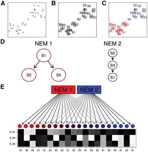
A schematic example of an M&NEM. Two dimensional projection of single cells (A), labeled by known knock-outs of signalling genes S1, S2 and S3 (B) and colored by their two clusters (C) on which the two different causal networks are based. (D) Comparing two different networks (NEMs) according to the clustering. S1, S2 and S3 are the perturbed genes and the edges denote how they causally influence each other. (E) 20 noisy cells attached to each NEM according to their responsibilities with their respective data patterns (black for effect and white for no effect). Each row shows the effect pattern for the respective S-gene, e.g. E_S1 shows the effects of S-gene S1 for different cells. Each column shows the expected data pattern for a cell. The colors and arrow transparencies depict the strength of attachment to the respective NEM. For example the bright red cell to the far left is attached to NEM 1 with responsibility 100%. Thus the pattern for the cell is the expected data pattern according to NEM 1 without any noise. The cells in the center are a mix of expected data patterns of cells for NEM 1 and NEM 2

We show that Mixture Nested Effects Models (M&NEMs) work well in the controlled setting of a simulation study and apply our method to three data sets from two different pooled CRISPR screens based on Crop-Seq (Datlinger et al., 2017) and Perturb-Seq (Dixit et al., 2016). In those screens, thousands of cells were pooled and each transfected with a different sgRNA to knock-out a specific gene. Gene expression data was generated by single-cell RNA-Seq. For the Crop-Seq screen we concentrated on one data set investigating the T-cell receptor pathway in the T-Cell leukemia derived Jurkat cell line and key regulators DOK2, EGR3, LAT, LCK, PTPN6, PTPN11 and ZAP70. From the Perturb-Seq screen we model the causal interplay of cell cycle genes in one data set and transcription factors in another data set. Both data sets of the Perturb-Seq screens are derived from K562 leukemia cells.

2 Model

In this section we review the original Nested Effects Model and extend it to a mixture of NEMs. Furthermore we discuss identifiability and propose a method for model selection to prevent over fitting.

2.1 Nested Effects Model

A Nested Effects Model (NEM) is parametrized by an adjacency matrix $\Phi \in M_{n\times n}(\left\{0,1\right\})$ for the directed acyclic graph (DAG) representation of the signaling graph with perturbed genes as nodes (S-genes) and an adjacency matrix $\Theta \in M_{n\times m}(\left\{0,1\right\})$ for the attachments of the different features from the data (E-genes), e.g. genes from gene expression data. We have ${\theta }_{ij}=1$⁠, if E-gene j is attached to S-gene i. Each column of Θ has at most one non-zero entry, because NEMs make the assumption that each E-gene can have at most one parent. Similar to Tresch and Markowetz (2008) we add a null S-gene, which predicts no effects to account for uninformative features.

We calculate the expected E-gene profiles for a given model $\left(\Phi ,\Theta \right)$ as the matrix product

$$F=\Phi \Theta$$

(1)

with f_ij the predicted state of E-gene i under knock-down of S-gene j.

Let $D=(d_{ij})\in M_{m\times l}(\mathbb{R})$ be the raw data matrix of the perturbation experiments and $R=(r_{ij})\in M_{m\times l}(\mathbb{R})$ the log ratio matrix with l perturbed cells or samples indexing the columns and m observed genes indexing the rows,

$$r_{ij}=\text{log}\frac{P(d_{ij}|e_{ij}=1)}{P(d_{ij}|e_{ij}=0)}.$$

with e_ij the unknown state of E-gene i in knock-down j. As in Tresch and Markowetz (2008) we can write the log likelihood ratio of a given model $\left(\Phi ,\Theta \right)$ and the null model N, which predicts no effects, as

$$\text{log}P(D|\Phi ,\Theta )-\text{log}P(D|N)=\text{tr}(L)$$

(2)

where $\text{tr}$ denotes the trace of the quadratic matrix of log ratios for all knock-downs and L = FR. However, L is only quadratic if the data includes only one sample per knock-down, i.e. l = n. Hence, the data has to be summarized beforehand, e.g. by taking the average over all experiments with the same knock-down (replicates).

2.2 Mixture Nested Effects Model

Instead of inferring a single network $\Phi$ and E-gene attachments Θ from the whole data set as in the previous section, we formulate a mixture, which infers several networks with unique attachments and different subpopulations of cells.

The model parameters for a mixture of K components are

$$\left(\Phi ,\Theta \right)={\left({\Phi }_k,{\Theta }_k\right)}_{k=1,\dots ,K}$$

and mixture weights $\pi =\left({\pi }_1,\dots ,{\pi }_K\right)$⁠.

Given a component $({\Phi }_k,{\Theta }_k)$ we calculate the expected knock-down profiles for all single perturbations using Eq. 1 as

$$F_k=(f_{k,ij})={\Phi }_k{\Theta }_k$$

with $f_{k,ij}$ the expected value of E-gene j under the perturbation of S-gene i in component k.

The log ratio profile of all cells given component k is

$$L_k=(l_{k,ij})=F_{k}R$$

and the log likelihood ratio of component k is

$$\text{log}P(D|F_k)-\text{log}P(D|N)=\text{tr}(L_k).$$

However, instead of summarizing each knock-down over all cells in R to make L_k quadratic, we use the known perturbation map $\rho =\left({\text{ϱ}}_{ij}\right)$ with ${\text{ϱ}}_{ij}=1$⁠, if cell j has been perturbed by a knock-down of S-gene i. We set

$${\tilde{L}}_k=\left({\tilde{l}}_{k,ij}\right)={\rho }^T{L}_k.$$

(3)

In this formulation, we have conveniently stored the likelihood ratios for all cells in the diagonal of ${\tilde{L}}_k$⁠.

Let $Z\in M_{K\times l}(\left\{0,1\right\})$ be the matrix of hidden cell attachments to components. We have z_ki = 1, if cell i belongs to component k. Each column of Z has exactly one non-zero entry. The distribution of Z is defined by the mixing coefficients π_k as

$$P(z_{ki}=1)={\pi }_k$$

for all $i\in \left\{1,\dots ,l\right\}$ with $\pi =({\pi }_1,\dots ,{\pi }_K)\in {\left[0,1\right]}^K$ and ${\displaystyle {\sum }_k{\pi }_k}=1$⁠.

For model optimization we choose a maximum likelihood (ML) approach using the log likelihood ratios similarly to the formulation for a single mixture component, and maximize

$$\begin{array}{c}\mathcal{L}=\text{log}P(D|\Phi ,\Theta )-\text{log}P(D|N)\\ =\text{tr}\left(\text{log}{\displaystyle \sum _{k=1}^K{\pi }_k}\text{exp}({\tilde{L}}_k)\right).\end{array}$$

(4)

The full derivation of the likelihood ratio is in Supplementary Eq. S1 of the supplement.

2.3 Inference with an Expectation maximization algorithm

We developed an Expected Maximization algorithm (Dempster et al., 1977) for inference.

E step. Let  $\left(\pi ,\Phi ,\Theta \right)$ be the current parametrization of our mixture model. We calculate ${\tilde{L}}_k$ from Eq. 3 and subsequently the responsibilities (supplement, Supplementary Eq. S2)

$$\gamma (z_{ki})=P(z_{ki}=1|d_i)=\frac{{\pi }_k\text{exp}\left({\tilde{l}}_{k,ii}\right)}{{\displaystyle {\sum }_{j=1}^K{\pi }_j}\text{exp}\left({\tilde{l}}_{j,ii}\right)},$$

(5)

which we summarize in

$$\Gamma =({\gamma }_{ki})\in M_{K\times l}(\left[0,1\right]).$$

and the log likelihood ratio (Eq. 4).

$M_{\Theta }$  step. We update π with

$${\pi }_k=\frac{{\displaystyle {\sum }_{i=1}^l{\gamma }_{ki}}}{{\displaystyle {\sum }_{j=1}^K{\displaystyle {\sum }_{i=1}^l{\gamma }_{ji}}}}$$

and compute

$$R_k=(r_{ij}{\gamma }_{kj}).$$

$\mathbf{\Phi }$ remains fixed and we estimate $\mathbf{\Theta }$ by their maximum a posteriori attachment to each S-gene. We compute the fit of every E-gene to every S-gene

$$P_k=\left(p_{k,ij}\right)=R_k{\rho }^T{\phi }_k$$

(6)

and set ${\theta }_{k,ij}=1$⁠, if $p_{k,ji}=\text{max}\left\{p_{k,jl}:l=1,\dots ,n\right\}$⁠.

We alternate between the E step and the $M_{\Theta }$ step until the log likelihood ratio in Eq. 4 converges.

M step. Given Γ, we optimize each component $({\Phi }_k,{\Theta }_k)$ with respect to R_k. We maximize the log likelihood ratio defined in Eq. 2 to find a new optimum $\left({\Phi }_k^{new},{\Theta }_k^{new}\right)$ in the following way.

We optimize each individual component with a natural extension of the module network approach by Frohlich et al. (2008). We cluster knock-downs, averaged over cells, into groups of size n (e.g. n = 5) and perform a local neighborhood search on each group. In the local neighborhood search we evaluate each edge for absence and presence and check whether a change in status improves the log likelihood ratio and change the edge which improves it most. We combine the inferred sub-networks into one large network including all S-genes and use it as the initial network for a local neighborhood search on the full set of S-genes. During the optimization of ${\Phi }_k$⁠, we estimate Θ_k using P_k (Eq. 6) before we calculate the log likelihood ratio.

We alternate between the E, $M_{\Theta }$ and M steps until the log likelihood ratio in Eq. 4 converges. To increase the probability of convergence to a global optimum, the EM algorithm is initialized several times with random responsibilities Γ between 0 and 1.

2.4 Model identifiability

In the case of the original NEMs, two NEMs ${\Phi }_1$ and ${\Phi }_2$ are identical if and only if they have equal transitive closures, i.e. they produce identical data. This identity still holds for each component of a mixture of NEMs. However, like any mixture model, M&NEMs have additional identifiability issues.

In general, two M&NEMs are not distinguishable, if they have the same expected data pattern. Let $F=\left(F_1,\dots ,F_m\right)$ be the expected data pattern for M&NEM A and $\tilde{F}=\left({\tilde{F}}_1,\dots ,{\tilde{F}}_n\right)$ the expected data pattern for M&NEM B. If each column f_v of F is included in $\tilde{F}$ and each column ${\tilde{f}}_w$ of $\tilde{F}$ is included in F, A and B are not distinguishable.

Figure 2 shows a schematic example for two different mixtures A and B, which both have the exact same expected data pattern. Hence, they also have the same likelihood ratio given any dataset. For convenience of this example we assume an a posteriori hard clustering of the cells to the components and equal attachments ${\Theta }_1={\Theta }_2$⁠.

Fig. 2.

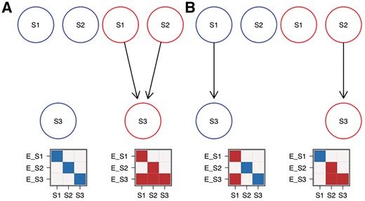
Example for non-identifiability of two M&NEMs. (A) Mixture of two components (blue, red) with their respective expected data patterns below. Dark areas are effects and light areas are no effects. Each column of the data is a cell and each row is the expected effect pattern for gene E_X attached to S-gene X. (B) Mixture with different components than A, but overall the exact same expected data profile

2.5 Model selection

In a typical situation for M&NEMs we do not know the correct number of components K, i.e. the number of subpopulations with different signaling networks. To prevent over fitting and enforce sparsity to the solution, we choose the optimal K via a penalized log likelihood ratio, penalizing complex and redundant network structures in a similar fashion as Froehlich et al. (2007). For each $K\in \left\{1,\dots ,5\right\}$ we infer an optimal solution using the EM algorithm. Then we score each of the five solutions with a penalized log likelihood ratio, which we define as

$$\tilde{\mathcal{L}}=\text{log}\left(n\right)s-2\mathcal{L}$$

(7)

with a complexity parameter s, model log likelihood ratio $\mathcal{L}$ (Eq. 4) and the sample size n (number of cells). We define s for a mixture of K components as

$$s={\displaystyle \sum _k\left(\left|{\Phi }_k\right|+\left|{\Theta }_k\right|\right)}+K-1$$

(8)

with number of edges of an adjacency matrix A denoted by $\left|A\right|$⁠. Thus the number of parameters s are all edges in the graphs of ${\Phi }_k$ and Θ_k plus one less than the number of mixture weights, since the last weight is determined by the others. Finally we choose the solution, which minimizes the penalized log likelihood ratio. Figure 3 shows the raw and the penalized log likelihood ratio as functions of the number of components for the data sets in our applications.

Fig. 3.

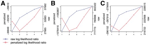
Penalized log likelihood ratio (red, left y-axis) in comparison with the raw log likelihood ratio (blue, right y-axis) as functions of number of components for the Crop-Seq regulators of the T-Cell receptor (A) and the Perturb-Seq cell cycle genes (B) and transcription factors (C)

2.6 Effect log-odds

We calculate log odds between the likelihood of observing an effect and observing no effect given the data analogous to Siebourg-Polster et al. (2015). Let d_ij be the normalized count value for gene i and cell j. Cell j was perturbed by a knock-down of gene k. We estimate the empirical distribution function F₀ of the normalized control counts for gene i and the empirical distribution function F_k of the normalized counts from cells perturbed by k for gene i and calculate the log odds by

$$r_{ij}=\text{log}\frac{P\left(d_{ij}|F_k\right)}{P\left(d_{ij}|F_0\right)}.$$

(9)

If the E-gene shows an effect in the cell, r_ij will be greater than zero and if it shows no effect, it will be less than or equal to zero.

We remove E-genes with a standard deviation of log odds smaller than the global standard deviation of log odds over the whole data set, i.e. E-genes which have small log odds apart from outliers.

3 Simulations

We show that M&NEMs work well in simulations under reasonable conditions, i.e. medium noise levels, up to 20 S-genes and five components. For $n\in \left\{3,5,10,20\right\}$ S-genes and $K\in \left\{1,2,3,4,5\right\}$ network components we drew random mixture weights π and component(s) $\left(\Phi ,\Theta \right)$ as the ground truth. We simulated 1000 cells overall, two E-genes per S-gene and 10% uninformative E-genes. The simulated data were log odds drawn from Gaussian distributions $\mathcal{N}\left(-1,\sigma \right)$ for no effect and $\mathcal{N}\left(1,\sigma \right)$ for effect. Figure 4 shows the result of 100 runs and $\sigma \in \left\{1,2.5,5\right\}$⁠. We applied M&NEM to the data with $K\in \left\{1,2,3,4,5\right\}$ and chose the best K according to the penalized log likelihood ratio (Eq. 7).

Fig. 4.

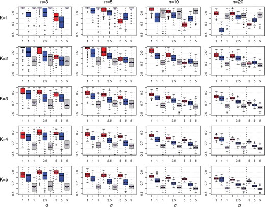
Comparison of M&NEMs (red), cNEMs (blue) and NEMs (grey) in a simulation study. The rows show results for components $K\in \left\{1,2,3,4,5\right\}$⁠. The columns show results for number of S-genes $n\in \left\{3,5,10,20\right\}$⁠. Each box plot shows the accuracy of M&NEM (red), cNEM (blue) and NEM (grey) for three different noise levels σ. The y-axis is cutoff at 50% (⁠$=$random). In addition to the median we also added the average (red star in blue circle)

We computed accuracy from similarity of the ground truth ${\Phi }^T=\left({\Phi }_1^T,\dots ,{\Phi }_K^T\right)$ and the inferred optimum ${\tilde{\Phi }}^T=\left({\tilde{\Phi }}_1^T,\dots ,{\tilde{\Phi }}_{\tilde{K}}^T\right)$⁠. That is, we check how accurately we find a column from the ground truth ${\Phi }^T$ in the inferred optimum ${\tilde{\Phi }}^T$ and vice versa with the following score,

$$\begin{array}{c}\text{A}\left({\Phi }^T,{\tilde{\Phi }}^T\right)=\min \{{\displaystyle \sum _{k=1}^K{\displaystyle \sum _{i=1}^n\underset{j=1,\dots ,\tilde{K}}{\max }}}\left\{\text{acc}\left({\phi }_{k,i},{\tilde{\phi }}_{j,i}\right)\right\},\\ {\displaystyle \sum _{k=1}^{\tilde{K}}{\displaystyle \sum _{i=1}^n\underset{j=1,\dots ,K}{\max }}}\left\{\text{acc}\left({\tilde{\phi }}_{k,i},{\phi }_{j,i}\right)\right\}\}\end{array}$$

with ${\phi }_{k,i}$ as column i of ${\Phi }_k^T,{\tilde{\phi }}_{j,i}$ as column i of ${\tilde{\Phi }}_j^T$ and

$$\text{acc}\left(u,v\right)=1-\frac{\text{hd}\left(u,v\right)}{\text{hd}\left(u,1-u\right)}$$

with the hamming distance $\text{hd}$⁠.

We compared M&NEMs to the original NEM and a naive cluster approach (cNEM). In cNEM we calculate the distance between cells from correlation and use K-means (⁠$K\in \left\{2,\dots ,5\right\}$⁠) to cluster the cells. We use the silhouette score to choose the optimal number of clusters and learn a single NEM on each cluster. The distance measure for two cells a, b is computed by

$$\text{dist}\left(a,b\right)=\frac{\left(1-\text{cor}\left(a,b\right)\right)}{2}.$$

The simulations show that M&NEMs can identify the ground truth with high accuracy for reasonable noise levels and is still robust in settings with high noise over a varying number of components and S-genes. For K = 1 M&NEM and NEM are equally successful in recovering the ground truth except for very high noise levels. For K > 1 M&NEM achieves a higher accuracy than cNEM, while the original NEM approach has the lowest accuracy especially for larger K. The accuracy for K and the mixture weights are shown in Supplementary Figures S1–S2.

4 Application to pooled single cell CRISPR screens

In our application of M&NEM to real data we analyze three data sets which combine pooled CRISPR screening with single cell RNA-seq readouts. One data set was generated with Crop-Seq (Datlinger et al., 2017) and the other two with Perturb-Seq (Dixit et al., 2016).

We preprocessed all data sets with Linnorm (Yip et al., 2017), which was specifically designed to normalize gene expression data from single-cell RNAseq (scRNA-seq) experiments. Linnorm accounts for typical noise expected in scRNA-seq data like random drop out events and zero inflated counts. After normalization we calculated the log odds (Eq. 9).

4.1 CRISPR droplet sequencing (Crop-Seq)

Datlinger et al. (2017) combined pooled CRISPR screening with single-cell RNA sequencing to produce gene expression count data on the single-cell level. They showed the validity of their method with an analysis of T-cell receptor (TCR) activation in Jurkat cells. We downloaded the processed CROP-seq data from the NCBI GEO database (Edgar et al., 2002, GSE92872). Before our analysis we reduced the data to stimulated cells.

As a set of knock-outs we concentrated on S-genes involved in T-Cell receptor activity as in Figure 2h of Datlinger et al. (2017), namely: DOK2, EGR3, LAT, LCK, PTPN6, PTPN11 and ZAP70. This leaves us with a population of 535 unique cells and 711 E-genes. Figure 5 shows the result for the highest scoring model with K = 2. Around 43% of cells are assigned to the red network and 57% to the blue one. M&NEM confirms key down-stream regulators LCK, LAT and ZAP70 for the red network (Datlinger et al., 2017, Fig. 2h). However, we never find LCK upstream of ZAP70. While LAT remains downstream, LCK and especially ZAP70 are placed more upstream in the blue network with ZAP70 as the only source node. DOK2 on the other hand is correctly placed as an upstream regulator in the red network (Datlinger et al., 2017, Fig. 2h), but placed downstream of everything else except LAT in the blue one. This hints at an altered causal roles of DOK2, LCK and ZAP70 in the larger cell population. PTPN6 and PTPN11 switch places and alternatively regulate each other and major parts of the other S-genes.

Fig. 5.

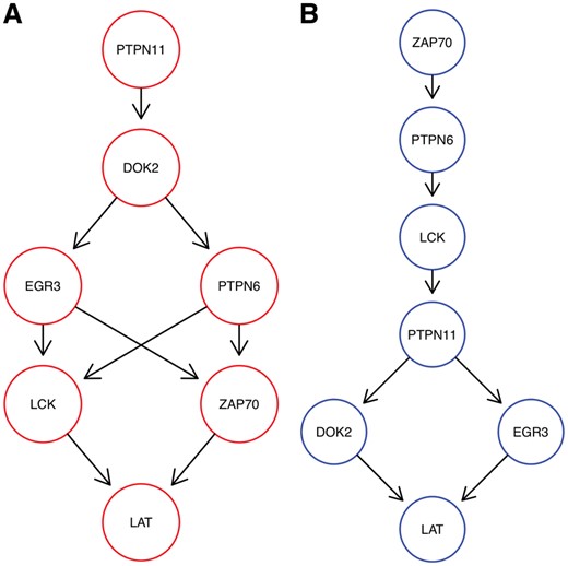
Optimal mixture found for the Crop-Seq data set (K = 2) with mixture weights 43.3% (A, red) and 56.7% (B, blue)

A posteriori a majority of 303 cells are attached to the blue network. However, for LCK, ZAP70 and PTPN6 the majority of cells for each knock-out are attached to the red network, which explains the relatively high mixture weight of 43%, The responsibilities for each network are almost binary, 100% respectively 0% (Fig. 6A). This is almost equivalent to a hard clustering of the cells, i.e. there is virtually no uncertainty of the cell attachments.

Fig. 6.

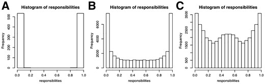
Histograms of responsibilities for Crop-Seq (A), Perturb-Seq cell cycle regulators (B) and transcription factors (C)

A more detailed version of the network for the three highest scoring models (⁠$K\in \left\{1,2,3\right\}$⁠) are shown in the supplement (Supplementary Figs S3–S5).

4.2 Combining CRISPR-based perturbation and RNA-seq (Perturb-Seq)

The data sets of Dixit et al. (2016) consist of RNA-seq transcriptome read-outs for single cells. We downloaded them from the BROAD single-cell portal (https://portals.broadinstitute.org/single_cell).

Cell Cycle Regulators.  Dixit et al. (2016) performed knock-out experiments for thirteen cell cycle regulators in K562 cells. After preprocessing, the data set consists of 19 283 cells and 985 E-genes. Figure 7 shows the highest scoring M&NEM result (K = 2) with mixture weights 45.1% (red) and 54.9% (blue). However, a posteriori only around 39% of cells are assigned to the red network.

Fig. 7.

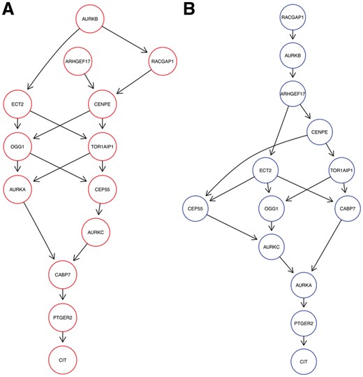
Optimal mixture found for the Perturb-Seq cell cycle regulators (K = 2) with mixture weights 45.1% (A, red) and 54.9% (B, blue)

Dixit et al. (2016) identified the perturbations of PTGER2, CAB7 and CIT as advantageous for proliferation. We found PTGER2 and CIT at stable positions downstream in both our networks, while CAB7 is placed a bit more upstream in the blue one. However, Dixit et al. (2016) found a distinct transcriptional phenotype for CAB7, which can explain the different roles in the networks in comparison to PTGER2 and CIT.

Reciprocally, perturbations of RACGAP1, TOR1AIP1 and AURKA were identified by Dixit et al. (2016) as disadvantageous to proliferation. However, while RACGAP1 stays almost right upstream in both, the other two are mostly placed in the middle. AURKA is even placed almost downstream of all other nodes in the blue network. This hints at much more diverse regulatory roles of the latter two and a necessity for RACGAP1 to stay upstream in the network as a key regulator (Imaoka et al., 2015).

Overall the networks differ also in their general shape. While the blue network has a more linear shape, the red network is much more inter-connected with two instead of one source node.

The histogram of responsibilities is shown in Figure 6B. The posterior attachment of cells shows a much softer gradient than for the Crop-Seq data set. While each S-gene in each component has at least one cell with responsibility $\ge 98$%, for many cells the responsibilities are between 5% and 95%. We show a more detailed depictions of the three highest scoring M&NEMs in the supplement (Supplementary Figs S6–S8).

Transcription Factor Interplay. In a second data set, Dixit et al. (2016) performed knock-out experiments for ten transcription factors in K562 cells. The preprocessed data set consists of 22 402 cells and 710 E-genes. Figure 8 shows the optimal network inferred by M&NEM (K = 2) with mixture weights of 45.2% (red) and 54.8%.

Fig. 8.

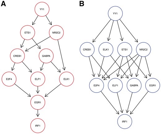
Optimal mixture found for the Perturb-seq transcription factors (K = 2) with mixture weights 45.2% (A, red) and 54.8% (B, blue)

We identify YY1 as a major regulator for all other genes as it is placed most upstream in both networks. YY1’s importance as a major transcription factor has been shown before (Tastanova et al., 2016). This is further confirmed as even M&NEM with more components (K = 3, supplement, Supplementary Fig. S10) still place YY1 most upstream in all networks. Similarly, the upstream causal relations of YY1 to NR2C2 and ETS1 is conserved as well. The position of IRF1 as the sink node is equally well conserved in both networks. The other transcription factors mainly stay in the middle part and only slightly switch places.

Again, the posterior attachment of cells shows a much softer gradient than for the CROP-seq data set (Fig. 6A and C). While each S-gene in each component has at least one cell with responsibility $\ge 98$%, for many cells the responsibilities are between 20 and 80%. However, we observe a large bump at 50%, which means many cells fit equally well to both networks. This agrees with our observation, that the causal network of transcription factors seems highly stable over all cells, compared to the other two applications before. This is further confirmed by our penalized log likelihood, which shows little support for K > 2 (Fig. 3C).

A more detailed depictions of the three highest scoring M&NEMs is shown in the supplement (Supplementary Figs S9–S11).

5 Discussion

We have introduced M&NEM, a novel method for the identification of heterogeneous subpopulations of single cells with different underlaying biological networks. M&NEM infers multiple networks from a heterogeneous cell population instead of a single one averaged over the whole population. This additional flexibility allows us to compensate model limitations of the original NEM. M&NEM successfully infers subpopulations and the underlaying mixture of networks.

In our application study, we have investigated three data sets from single cell CRISPR experiments combined with full transcriptomic read-outs. M&NEM confirms known causal interactions and infers novel ambiguous roles for several key regulators (e.g. DOK2, ZAP70), which might be differently regulated in a subpopulation of cells. We also identify key players like RACGAP1 and YY1, which seem to be necessary for upstream regulation.

Without the use of our model selection to enforce sparseness, our model might lead to over fitting. However, this over fitting might not always be due to noise or technical artifacts, but could also be due to hidden players not perturbed in the data as proposed by Sadeh et al. (2013). For example, if we look at the second highest scoring M&NEM for the cell cycle regulators (K = 3, supplement, Supplementary Fig. S7), we see that AURKA is placed downstream of the blue network with no cells attached and the highest responsibility for a cell at 10%, i.e. very little information for this placement of the AURKA S-gene comes from a cell in which AURKA was perturbed. Our hypothesis is that many E-genes react to PTGER2 and many E-genes react to CIT, but also many E-genes react to both. Original NEMs cannot model this and it is the exact situation for which Sadeh et al. (2013) introduced a hidden player (not perturbed) to account for the diversity of E-genes. In our blue network, AURKA is placed to model the unknown hidden player and not the actual AURKA S-gene (Fig. 9). However, Sadeh et al. (2013) use a binomial test based on the binarized data to account for noise, while our model does it in a greedy fashion, which we penalize with our penalized log likelihood ratio. Hence, an integration of the method of Sadeh et al. (2013) into our mixture model to identify hidden players accounting for noise would be an interesting addition.

Like any mixture model M&NEM suffers from identifiability issues. However, our simulations have shown that M&NEMs can still accurately predict the causal edges within a mixture of networks.

Fig. 9.

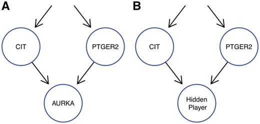
M&NEMs use a degree of freedom to model the possible location of a hidden player not included into the experimental design. The subgraph A shows the M&NEM result with a sink node not supported by any cells and the subgraph B shows our hypothesis for the location of an unperturbed hidden player

Funding

Part of this work was funded by SystemsX.ch, the Swiss Initiative in Systems Biology, under Grant No. RTD 2013/152 (TargetInfectX – Multi-Pronged Perturbation of Pathogen Infection in Human Cells), evaluated by the Swiss National Science Foundation.

Conflict of Interest: none declared.