


Abstract
Genomewide position-specific scores, such as those estimating conservation, constraint, fitness or mutation tolerance, are ubiquitous in current genome analyses. The diversity of sources and formats of these scores, as well as their size, increase the burden to use them. We present GenomicScores, a Bioconductor package that provides efficient storage and seamless access of genomewide position-specific scores from R, facilitating their use in genome analysis workflows.
GenomicScores is implemented in R and available at https://bioconductor.org/packages/GenomicScores under the open source ‘Artistic-2.0’ license.
Supplementary data are available at Bioinformatics online.
1 Introduction
Genome-wide position-specific scores assign each genomic position a numeric value typically measuring conservation, constraint, fitness or mutation tolerance. Genomic scores are built on the basis of different sources of information such as sequence homology, functional domains or physicochemical changes of amino acid residues, among others. These scores are widely used to filter single nucleotide variants or assess the degree of functionality of genome features. One particular and widely used instance of genomic scores are phastCons scores providing a measure of conservation calculated from genomewide alignments (Siepel et al., 2005).
However, retrieving, parsing and integrating diverse genomic scores often becomes a cumbersome task due to the multiple sources and formats of storage, as well as the size of the files that contain them, which grows substantially in the case of genomes of higher eukaryotes. The GenomicScores package addresses this problem to facilitate an efficient storage and seamless access of these scores, and their integration into genome analysis workflows on top of R and Bioconductor (Huber et al., 2015). The GenomicScores software package, and others used in this article through the call to the R function library(), can be installed in Linux, Windows or Mac OSX, by following the instructions available at https://bioconductor.org/install. The functionality illustrated in this article forms part of the Bioconductor release version 3.7 and it is more comprehensively documented in the online manual and vignette included in the software.
2 Results
Storing and accessing genomic scores is challenging when their values cover large regions of the genome, resulting in gigabytes of double-precision numbers. This is the case, for instance, of phastCons (Siepel et al., 2005), CADD (Kircher et al., 2014) or M-CAP scores (Jagadeesh et al., 2016). We address this problem by using lossy compression, storing quantized scores with run-length encoding (RLE) compressed vectors. Lossy compression attempts to trade off precision for compression without compromising the scientific integrity of the data (Zender, 2016). Limiting numeric precision leads to a subset of quantized values much smaller than the original range of genomic scores. This enables using only one or two bytes of storage for each score, and leads to long runs of identical values along the genome that can be compressed with RLE vectors; see Supplementary Note and Figure S1.
We have processed in this way a number of genomic score sets, rounding off the original values to 1 or 2 decimal places, or significant figures; see Supplementary Tables S1–S3. The GenomicScores package exposes these scores to the user through the object class GScores, which jointly with its associated methods, is designed with three goals. First, retrieve metadata including versioning, provenance and citation data. Second, minimize the memory footprint by loading only the scores associated with the queried genomic sequences. Third, provide a common access point through the functions gscores() and score(). The following example shows a basic use case where we query the phastCons average score for the genomic range 117, 232, 380–117, 232, 384 in the human chromosome 7.
> library(GenomicScores)
> library(phastCons100way.UCSC.hg19)
> phast <- phastCons100way.UCSC.hg19
> phast
GScores object
# organism: Homo sapiens (UCSC, hg19)
# provider: UCSC
# provider version: 09Feb2014
# download date: Apr 10, 2018
# loaded sequences: chr19_gl000208_random
# number of sites: 2858 millions
# maximum abs. error: 0.05
# use ’citation()’ to cite these data in publications
> gscores(phast, GRanges(“chr7: 11834150-11834154”))
GRanges object with 1 range and 1 metadata column:
seqnames ranges strand | default
<Rle> <IRanges> <Rle> | <numeric>
[1] chr7 11834150-11834154 * | 0.2
——-
seqinfo: 1 sequence from unspecified genome; no seqlengths
Using a GRanges object (Lawrence et al., 2013) we queried a single genomic range of positions for which the mean score was calculated, but we can retrieve other summary statistics such as minimum or median values with the argument summaryFun. By default, the gscores() method returns the scores in a GRanges object but it can return them as a numeric vector by using the function score() instead.
> score(phast, GRanges(“chr7: 11834150-11834154”))
[1] 0.2
The previous example loads a Bioconductor annotation package (phastCons100way.UCSC.hg19) that stores phastCons genomic scores. Other Bioconductor annotation packages storing genomic score sets are listed in Supplementary Table S1. Among them, those whose name starts with the MafDb prefix provide minor allele frequency (MAF) data. Some score sets may be formed by different scores populations, corresponding to different precision levels (e.g. rounding off to 1 or 2 decimal places) or different data sources from which the scores were derived (e.g. MAF data derived from different human populations). To find out the available scores populations available in each score set, we can use the function populations(), and to use a specific one we can use the argument pop where appropriate.
> populations(phast)
[1] “default” “DP2”
> score(phast, GRanges(“chr7: 11834150-11834154”), pop=“DP2”)
[1] 0.214
Additional genomic scores sets (Supplementary Table S2) are also available online as AnnotationHub resources (Morgan, 2017) that can be retrieved as follows:
> availableGScores()
[1] “cadd.v1.3.hg19” “fitCons.UCSC.hg19”
[3] “linsight.UCSC.hg19” “mcap.v1.0.hg19”
[5] “phastCons7way.UCSC.hg38” “phastCons27way.UCSC.dm6”
[7] “phastCons60way.UCSC.mm10” “phastCons100way.UCSC.hg19”
[9] “phastCons100way.UCSC.hg38” “phyloP60way.UCSC.mm10”
[11] “phyloP100way.UCSC.hg19” “phyloP100way.UCSC.hg38”
> cadd <- getGScores(“cadd.v1.3.hg19”)
> mcap <- getGScores(“mcap.v1.0.hg19”)
Genomic score sets downloaded as AnnotationHub resources are cached on disk, so that a subsequent call to getGScores() on a previously downloaded score set, will just load it from disk. We illustrate below a use case of GenomicScores to find the top-3 most conserved single nucleotide variants in coding regions with largest deleterious effects predicted by CADD (Kircher et al., 2014) and M-CAP scores (Jagadeesh et al., 2016), and their gnomAD MAF values (Lek et al., 2016). For this purpose, we use the VariantAnnotation package (Obenchain et al., 2014) and one of its sample VCF files. Figure 1 shows a graphical representation of all the retrieved scores.
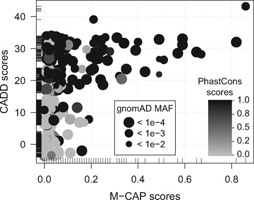
Relationship between CADD, M-CAP, PhastCons scores and gnomAD MAF values for variants from coding regions of chromosome 22. Values on the y-axis are jittered to improve visualization. Short lines along each axis are a 1-d representation of the axis data to visualize values that are present in one axis only. No dots are hidden behind the legends
> library(MafDb.gnomAD.r2.0.1.hs37d5)
> library(VariantAnnotation)
> library(TxDb.Hsapiens.UCSC.hg19.knownGene)
> mafdb <- MafDb.gnomAD.r2.0.1.hs37d5
> txdb <- TxDb.Hsapiens.UCSC.hg19.knownGene
> fl <- system.file(“extdata”, “chr22.vcf.gz”,
package=“VariantAnnotation”)
> vcf <- readVcf(fl, “hg19”)
> vcf <- vcf[isSNV(vcf)]
> seqlevelsStyle(vcf) <- seqlevelsStyle(txdb)
> loc <- unique(locateVariants(vcf, txdb, CodingVariants()))
> loc$PHAST <- score(phast, loc)
> loc$CADD <- score(cadd, loc, ref = ref(vcf)[loc$QUERYID],
alt = alt(vcf)[loc$QUERYID])
> loc$MCAP <- score(mcap, loc, ref = ref(vcf)[loc$QUERYID],
alt = alt(vcf)[loc$QUERYID])
> seqlevelsStyle(loc) <- seqlevelsStyle(mafdb)
> loc$MAF <- score(mafdb, loc)
> loc[order(loc\textit{PHAST}, \textit{loc}CADD, loc$MCAP, na.last = NA,
decreasing = TRUE)[1: 3], ]
GRanges object with 3 ranges and 13 metadata columns:
seqnames ranges strand | LOCATION LOCSTART
<Rle> <IRanges> <Rle> | <factor> <integer>
[1] 22 50699625 - | coding 226
[2] 22 50927976 + | coding 652
[3] 22 50689460 -| coding 2
LOCEND QUERYID TXID CDSID
<integer> <integer> <character> <IntegerList>
[1] 226 5615 75274 218661
[2] 652 8788 74392 216419, 216418
[3] 2 5450 75268 218646
GENEID PRECEDEID FOLLOWID
<character> <CharacterList> <CharacterList>
[1] 6300 <NA> <NA>
[2] 55586 <NA> <NA>
[3] 83933 <NA> <NA>
PHAST CADD MCAP MAF
<numeric> <numeric> <numeric> <numeric>
[1] 1 40 0.86 4e-04
[2] 1 40 0.21 0.001
[3] 1 30 0.82 3e-05
——-
seqinfo: 1 sequence from unspecified genome; no seqlengths
3 Conclusion
The GenomicScores package facilitates the integration of genomic scores into genome analysis workflows on top of R and Bioconductor. Additional score sets can be added on request at the Bioconductor support site (https://support.bioconductor.org). The underlying storage and representation of the serialized lossy-compressed genomic scores are RDS files (R Core Team, 2018, p. 12). This precludes the interoperability with platforms other than R, if a developer wants to access directly the content of those files from those platforms. However, because the access to the scores within R is achieved through an object class built on top of other Bioconductor data structures, improvements on compressing and distributing the scores can be made without breaking R code from end-users and other packages importing the GenomicScores functionality.
Acknowledgements
We would like to thank the Bioconductor core team for their technical support to implement some of the features of GenomicScores, and the two anonymous reviewers for their constructive comments that have improved this paper.
Funding
This work was supported by Spanish MINECO/FEDER (TIN2015-71079-P) and ‘Maria de Maeztu Unit of Excellence’ (MDM-2014-0370), and Catalan AGAUR (SGR17-1020; FI-DGR 2015).
Conflict of interest: none declared.
References

