In silico read normalization using set multi-cover optimization

Abstract

Motivation

De Bruijn graphs are a common assembly data structure for sequencing datasets. But with the advances in sequencing technologies, assembling high coverage datasets has become a computational challenge. Read normalization, which removes redundancy in datasets, is widely applied to reduce resource requirements. Current normalization algorithms, though efficient, provide no guarantee to preserve important k-mers that form connections between regions in the graph.

Results

Here, normalization is phrased as a set multi-cover problem on reads and a heuristic algorithm, Optimized Read Normalization Algorithm (ORNA), is proposed. ORNA normalizes to the minimum number of reads required to retain all k-mers and their relative k-mer abundances from the original dataset. Hence, all connections from the original graph are preserved. ORNA was tested on various RNA-seq datasets with different coverage values. It was compared to the current normalization algorithms and was found to be performing better. Normalizing error corrected data allows for more accurate assemblies compared to the normalized uncorrected dataset. Further, an application is proposed in which multiple datasets are combined and normalized to predict novel transcripts that would have been missed otherwise. Finally, ORNA is a general purpose normalization algorithm that is fast and significantly reduces datasets with loss of assembly quality in between [1, 30]% depending on reduction stringency.

Availability and implementation

ORNA is available at https://github.com/SchulzLab/ORNA.

Supplementary information

Supplementary data are available at Bioinformatics online.

1 Introduction

With increasing throughput and decreasing prices of modern sequencers, the generation of high coverage sequencing datasets has become routine. This has spurred the development of a number of different approaches for the de novo assembly of genomes and transcriptomes (Miller et al., 2010; Moreton et al., 2016). However, assembling a large genome or a transcriptome is a resource-intensive task.

Due to the large size of the datasets one particular line of research has focused on making data structures for de novo assembly more space-efficient for one or several datasets as applied to genome and metagenome sequencing (Chikhi et al., 2016; Pell et al., 2012). Another approach called compressed genomics deals with finding a compressed representation of the dataset to speedup computations, which was successfully applied to read alignment and SNP calling (Berger et al., 2013; Loh et al., 2012).

Here, we investigate how data reduction approaches affect the performance of non-uniform RNA-seq datasets for the task of de novo transcriptome assembly. This is an important problem as current assembly methods, which rely on the de Bruijn graph (DBG), consume a lot of main memory (Grabherr et al., 2011; Robertson et al., 2010; Schulz et al., 2012). However, it is also an interesting question from the perspective of information theory. Which parts of the data are actually being used by the assembler?

A simple approach to remove sequencing errors and reduce data size is to trim read suffixes and prefixes that are of low quality. This generally leads to decreased assembly performance (MacManes, 2014; Mbandi et al., 2014) and does not address the high redundancy of current read datasets. Other approaches allow the efficient correction of sequencing errors in RNA-seq datasets, which generally leads to an improved assembly performance (Le et al., 2013; Song and Florea, 2015), albeit at increased runtime because the data has to be error corrected (EC) first.

A direct approach to remove redundancy is to cluster reads according to sequence similarity using algorithms like CD-HIT (Fu et al., 2012) and remove highly similar reads in the clusters. Though recent improvements have been made for clustering assembled transcripts (Srivastava et al., 2016), clustering hundred millions of reads before assembly is still challenging.

Another widely used approach, in particular in combination with assembly, has been ‘digital normalization’ (Diginorm; Brown et al., 2012), implemented in the khmer package (Crusoe et al., 2015). Diginorm uses a min-count-sketch data structure to estimate k-mer abundance while streaming through the read dataset. Using a user-selected abundance threshold t, reads are removed once their median k-mer coverage goes beyond t. An idea similar to this is Trinity’s in silico normalization (TIS) which is a part of the Trinity assembler package (Haas et al., 2013). For each read in the dataset, TIS computes the median coverage of the k-mers in the read. If the median coverage is less than the desired coverage, the read is always kept. Otherwise, it is kept with a probability which is equal to the ratio of the desired coverage and the median coverage. Additionally, a read is removed if the ratio of SD of k-mer coverage to the average k-mer coverage of the read is higher than a cutoff. The recently developed NeatFreq algorithm (McCorrison et al., 2014) clusters the read into bins based on median k-mer frequency.

The advantage of k-mer coverage based normalization is 3-fold: (i) reads with high redundancy are removed leading to reduced memory and runtime requirements for the assembly, (ii) erroneous reads may be removed as part of the process and (iii) normalization is fast and consumes only a fraction of the memory an assembler would take. This essentially lowers the computational complexity of the assembly problem as it was shown that often a large part of the data can be removed, without significantly affecting assembly performance (Brown et al., 2012; Haas et al., 2013). However, previous algorithms do not give any certainty on preserving important parts of the data containing useful k-mers. Reads that contain low-abundant but important k-mers may be removed. This might result in losing connections in the DBG and hence a fragmented assembly might be generated. This is especially problematic for sequencing datasets with non-uniform coverage, like RNA-seq and metagenomics.

Here, the Optimized Read Normalization Algorithm (ORNA) is suggested based on the idea that reads are reduced without losing the DBG backbone (unweighted nodes and edges) and relative node abundances are preserved in the reduced dataset as compared to the original DBG. Given a set of n reads, where each read consists of m k-mers, read normalization is phrased as a set multi-cover (SMC) optimization problem on reads. In this work, a $\mathcal{O}(nm\hspace{0.17em}\text{log}\hspace{0.17em} (nm))$ time heuristic algorithm is suggested that is shown to work well in practice. Analysis of normalized and EC data reveal that better assemblies can be produced with significant savings in runtime and memory consumption. The software is freely available at https://github.com/SchulzLab/ORNA under an MIT license.

2 Materials and methods

2.1 Problem formulation

A dataset $\mathcal{R}=\{r_1,r_2,\dots ,r_n\}$ is a set of n reads where each read is a sequence of DNA bases of fixed length s. Each read consists of a set of short words (k-mers) of length k. Most of the de novo assemblers start by constructing a DBG. k-mers obtained from all the reads in $\mathcal{R}$ are considered as vertices. Two vertices are connected by an edge if they overlap by k – 1 bases. Each edge is identified by a unique label l of length k + 1, such that the source vertex is a prefix of l and the destination vertex is a suffix of l. Since the labels are also generated from the reads in the dataset, each read $r\in \mathcal{R}$ can be considered as a set of $m=s-k$ labels, i.e. $r=(l_1,l_2,\dots ,l_m)$⁠, where l_i is a k + 1-mer obtained from the ith position in read r.

The objective of a normalization algorithm is to reduce the data as much as possible without having significant impact on the quality of the assembly produced. Since an assembly is produced by traversing paths in the DBG, it may be worthwhile that a new DBG build from the normalized dataset preserves all the (unweighted) nodes and edges of the original graph. Further, normalization should maintain the relative difference of abundance between k-mers to resolve complex graph structures.

Here, we suggest to phrase read normalization as a SMC problem, defined as follows:

Instance: A dataset $\mathcal{R}$ of n reads, a set of k + 1-mers (defined as labels) L obtained from $\mathcal{R}$ such that $\underset{r\in \mathcal{R}}{\cup }r=L$ and a weight $w_l\ge 1$ for every $l\in L$⁠. Note that, each read $r\in \mathcal{R}$ is considered here as a set of labels.

Valid solutions:  $\mathcal{R}\prime \subseteq \mathcal{R}$ such that $\underset{r\in R\prime }{\cup }r=L$ and $\forall l\in L,\text{abund}(l,\mathcal{R}\prime )\ge w_l$ where $\text{abund}(l,\mathcal{R}\prime )$ denotes the number of occurrences of l in $\mathcal{R}\prime$⁠.

Objective:  $\text{Minimize}\hspace{0.17em}|\mathcal{R}\prime |$⁠.

This SMC formulation seeks to find the smallest set of reads, that covers all labels and satisfies all label weights w_l. The SMC problem was shown to be a NP-hard problem (Chekuri et al., 2012). A common approximation approach for the SMC problem, is the following greedy approach: an element in the universe is termed as active if it has not yet been covered by any of the selected sets. Cost-effectiveness of a set, to be considered for selection, is measured in terms of the number of active elements present in the set. The algorithm would iterate over sets and select the one which is the most cost-effective. In the scope of this work, each read represents a set of labels. Thus, a data structure has to be maintained that holds the reads in an order starting from the one which has the largest number of active labels. This order has to be updated after every iteration. Thus, given a dataset containing n reads, the greedy approach would take $\mathcal{O}(n^{2}m\hspace{0.17em}\text{log}(nm))$ time, where m is the number of labels in a read. The estimate is under the assumption that the reads are sorted by cost-effectiveness using a binary heap or a similar data structure, which is not efficient enough for the large datasets considered here.

2.2 ORNA

In this work, a different heuristic algorithm based on a greedy read selection strategy is used, in which the ordering of reads based on cost-effectiveness is ignored to save runtime. The approach is summarized in algorithm 1. A set $\mathcal{R}$ of n reads and a k-mer size k is given as input. Each read in $\mathcal{R}$ consists of m labels. Since each edge label is a k + 1-mer, all the possible $k\prime =k+1$-mers are obtained from the reads and are stored in a bloom filter using the BuildBloom (⁠$\mathcal{R},\hspace{0.17em}k\prime$⁠) function (line 3). This functionality is implemented using the GATB library (Drezen et al., 2014), which uses the BBHash algorithm for building a minimal perfect hash function (Limasset et al., 2017) after counting the k-mers with the DSK algorithm (Rizk et al., 2013). k-mer counting and storing the information requires $\mathcal{O}(nm\hspace{0.17em}\text{log}(nm))$ time. A counter array NodeCounter is maintained for each entry in the bloom filter and is initialized to zero (line 5). This operation requires $\mathcal{O}(nm)$ time.

The dataset is then iterated and each read in the dataset is checked whether it contains a $k\prime$-mer that needs to be covered. This is done by first collecting a set $V\prime$ of all the $k\prime$-mers in the read using the $ObtainKmers(r,k\prime )$ function (line 8). For each $k\prime$-mer in $V\prime$⁠, the corresponding weight is calculated using the ObtainWeight function (line 11). The node counter for the $k\prime$-mer is then checked and incremented if its current value is less than the given weight (line 12–15). A read is accepted if it contains at-least one $k\prime$-mer for which the corresponding counter is incremented otherwise it is rejected (line 17–19). Steps 7–20 require $\mathcal{O}(nm)$ time. All the accepted reads then denote the normalized dataset ${\mathcal{R}}_{\text{out}}$ obtained from $\mathcal{R}$⁠. The overall time complexity of the algorithm is $\mathcal{O}(nm\hspace{0.17em}\text{log}\hspace{0.17em} (nm))$⁠.

Algorithm 1

SMC based approach for read normalization

1: Input: Reads $\mathcal{R}$⁠, kmer size k

2: $k\prime =k+1$

3: V = BuildBloom(⁠$\mathcal{R},\hspace{0.17em}k\prime$⁠)

4: t = NumberOfkmers(V)

5: NodeCounter[1…t]$\leftarrow$0

6: ${\mathcal{R}}_{\text{out}}=\varphi$

7: for all$r\in R$do

8:   $V\prime$ = ObtainKmers(r,$k\prime$⁠)          ▹ $V\prime \subseteq V$

9:   flag = 0

10:    for all$v\in V\prime$do

11:     w = ObtainWeight(v, $\mathcal{R}$⁠)

12:     ifNodeCounter(v) < wthen

13:      NodeCounter(v) = NodeCounter(v) + 1

14:      flag = 1

15:     end if

16:    end for

17:    if$flag==1$then

18:     ${\mathcal{R}}_{\text{out}}={\mathcal{R}}_{\text{out}}\cup r$

19:    end if

20: end for

21: Output: Reads ${\mathcal{R}}_{\text{out}}$

An important parameter for the algorithm is the weight for each $k\prime$-mer. A naive way to decide the weight for each $k\prime$-mer is to set the same value for each. A DBG based assembler uses k-mer abundance information to resolve irregularities in the graph such as bubbles and tips. This information is also used for RNA-seq data to decide which transcripts should be reported. Hence, it is important to retain the relative difference in abundance between k-mers, which cannot be achieved with a fixed weight for all $k\prime$-mers. Therefore, each $k\prime$-mer has its own weight $w_{k\prime }$⁠, which is defined as:

$$\forall k\prime \in V\prime ,w_{k\prime }=\lceil \hspace{0.17em}{\text{log}}_b(\text{abund} (k\prime ,\mathcal{R}))\rceil ,$$

(1)

where $\text{abund} (k\prime ,\mathcal{R})$ is the abundance of $k\prime$ in $\mathcal{R}$⁠. b is the base of the logarithm function and is given by the user.

2.3 Normalization for paired-end data

For paired-end (PE) datasets ORNA is run in two passes. As in the single end mode, the dataset is iterated sequentially and only one pair is evaluated at a time. In the first pass, reads of a pair are checked for their acceptance. The pair is accepted only if both the reads of the pair satisfy the acceptance condition, i.e. there is at least one $k\prime$-mer in both the reads which needs to be covered in the normalized dataset. If only one read of the pair is satisfying the condition then the pair is marked, otherwise the pair is rejected. The counter for the $k\prime$-mers of marked pairs are not incremented at this point. Thus, the first pass might leave some $k\prime$-mers not covered in the normalized dataset. To cover such $k\prime$-mers, in the second pass, the marked pairs are again checked for acceptance and a pair is accepted if one of the reads satisfies the acceptance condition.

2.4 Data retrieval and normalization

Seven different datasets were used for the analyses shown in this work. Two datasets were downloaded from the SRA database- Brain dataset (Barbosa-Morais et al., 2012, SRR332171) which consists of 147 M PE reads with read length 50bps and hESC dataset (Au et al., 2013, SRR1020625) which has 142 M PE reads with length 50 bps. The datasets were EC, unless otherwise stated, using SEECER version 0.2 (Le et al., 2013) with default parameters. Further, a combined dataset of 883 M reads of length 76 bps was obtained by concatenating five ENCODE datasets: 101 M PE reads from hESC (GSM758573), 192 M PE reads from AG04450 (GSM765396), 207 M PE reads from GM12878 (GSM758572), 165 M PE reads from A549 (GSM767854) and 216 M PE reads from HeLa (GSM767847). The datasets were then normalized using ORNA (v0.2), Diginorm (v2.0) and TIS (v2.4.0) with parameter settings (see Supplementary Tables S1– S3 for parameter settings).

2.5 Transcriptome assembly and evaluation

To analyse the quality of the assembly produced from the reduced datasets, three DBG based de novo assemblers–Oases (Schulz et al., 2012, version 0.2.08), TransABySS (Robertson et al., 2010, version 1.5.3) and Trinity (Grabherr et al., 2011, version 2.4.0) were used. The assemblers were run with default parameters except the k-mer parameter of TransABySS and Oases. TransABySS was run using a single k-mer size (k = 21). Oases was run using multiple k-mer sizes (k = 21 to k = 49 with an increment of 2) and the assemblies obtained from all k-mer sizes were merged using the Oases merge-script.

The assembled transcripts were evaluated using the REF-EVAL program, which is part of the Detonate (Li et al., 2014, version 1.11) package, which is explained briefly. First, a true assembly for each dataset (Brain and hESC) was estimated, which estimated all regions from the reference transcript sequences (Ensembl) overlapped by reads. Second, the true assembly was bidirectionally aligned against the generated assemblies using Blat (Kent, 2002, version 36) and nucleotide precision and recall was obtained. REF-EVAL then reports the F1 score, which is the harmonic mean of the nucleotide precision and recall, as a measure of assembly accuracy. To measure the assembly contiguity, the assembled transcripts were aligned against a reference genome using Blat and the overlap was matched against annotated Ensembl transcripts downloaded from the Ensembl database (Cunningham et al., 2015, version 65). The number of Ensembl transcripts that were fully assembled by at least one distinct assembled transcript was obtained and termed as full-length transcripts.

For the analysis of the combined dataset, ORNA was used for normalization. The goal of the analysis was to determine how many transcripts are missed by assembling individual datasets, but are assembled using the combined datasets. All assemblies for this experiment were run with TransABySS (k = 21). The assembly generated by using all datasets was termed combined assembly. Individual dataset assemblies were clustered with the combined assembly using CD-HIT-EST (Fu et al., 2012, v4.6.4-2015-0603). Similar sequences were clustered together (sequence identity = 99%). Hence, if a transcript in the combined assembly is also assembled by any of the individual datasets, then it would be clustered with the sequences assembled from that dataset. All clusters which contained only the sequences from the combined assembly were termed as missed clusters and the longest sequence of the cluster was considered a missed transcript. Aligned missed transcripts were compared to annotations from Ensembl (Cunningham et al., 2015, version 65) and GENCODE (Harrow et al., 2012, version 17).

2.6 Correlation analysis

Further, gene expression values of all RNA-seq datasets for Ensembl transcripts were obtained using Salmon (Patro et al., 2017, v0.8.2). The k-mer parameter was set to 21 for quantification. Salmon provides quantification results at transcript level. To obtain the quantification at gene level, Transcripts Per Million (TPM) values of all the transcripts for a gene were summed. Spearman’s rank correlation values between original and reduced datasets were computed using the statistical computing language R (R Development Core Team, 2008, version 3.1.1).

3 Results

3.1 Comparison to established normalization algorithms

The task of a read normalization algorithm is to remove the maximum number of reads without compromising the quality of the assembly produced. Most of the de novo assemblers start by building a DBG using a fixed/variable k-mer size and generate assemblies by traversing paths in the graph. In order to maintain assembly quality, ORNA was designed to: (i) retain all nodes and their connections in the DBG and (ii) retain the relative abundance difference between k-mers in the reduced dataset.

Diginorm and TIS normalization base their decision on the k-mer abundance distribution within individual reads. A read might get removed if the median abundance of k-mers present in the read exceeds a certain threshold. Hence a k-mer having low abundance, if present among high abundance k-mers in the read, is also removed. For instance, Figure 1 shows a toy DBG. Nodes in the graph represent k-mers and the abundance of each node is represented as a number inside the node. If the desired median abundance is 10 then read r₁ covering node A, C, E and G would be removed since the median abundance of k-mers in r₁ is 20. Although, this strategy may potentially remove erroneous k-mers, it might also result in the loss of true k-mers which form connections between nodes in the graph. For instance, removal of read r₁ in the above example would remove the k-mer corresponding to node E (dashed node). Hence, the connection between node C and node G is lost, which possibly results in a fragmented assembly.

Fig. 1.

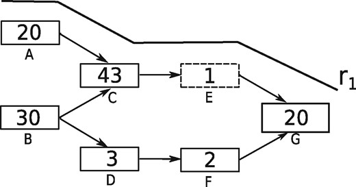
A toy DBG with one traversing read shown denoted r₁. Nodes in the DBG represent k-mers, numbers inside nodes represent the abundance of the corresponding k-mer in the data. Dashed node represents the k-mer, which will be lost if r₁ is removed

ORNA retains all the kmers from the original dataset. In this work, all the assemblies used for evaluation are generated by constructing a DBG, which uses a k-mer size of 21 (except for Trinity which always uses k-mer size 25). Hence the size of the edge label would be k + 1. Figure 2a shows the retention of 22-mers in reduced versions of the brain dataset by ORNA, Diginorm and TIS. Diginorm and TIS loose 2–10% of the 22-mers. ORNA considers the normalization problem as a SMC problem. The set of all possible edge labels (of length k + 1) serves as the universe. A single read is considered as a set of k + 1-mers and a dataset is considered as a collection of such sets. ORNA selects the minimum number of reads, which is required to cover all the elements of the universe a certain number of times. Hence, all edge labels from the original dataset are retained.

Fig. 2.

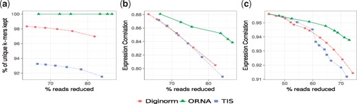
Comparison of k-mer information retained by ORNA, Diginorm and TIS. (a) Represents percentage of unique k-mers retained compared to the original brain dataset (x-axis) for various levels of reduction (y-axis) by the three algorithms. (b) and (c) Represent Spearman’s rank correlation values for TPM values obtained by quantifying expression of Ensembl genes using the unreduced and reduced brain dataset and hESC dataset, respectively

ORNA maintains the relative difference of abundance between k-mers. A de novo assembler generally uses the k-mer abundance information to resolve erroneous graph structures like bubbles and tips, among other things. For instance, in Figure 1, assume that a bubble is formed by nodes C, D, E and F. An assembler would remove this by converting the less abundant path B-D-F-G to the higher abundant path B-C-E-G. Hence, it is important to maintain the relative abundance difference between the k-mers. ORNA uses the log_b of the abundance of the connection (k + 1-mer) in the original dataset. This results in large reduction of highly abundant k-mers and little to no reduction of lowly abundant k-mers, maintaining relative abundance differences. Figure 2b and c show the comparison of Spearman’s rank correlation values obtained between TPM values of the reduced and unreduced brain and hESC dataset, respectively. It can be seen that in all cases, the correlation is either similar or higher for ORNA reduced datasets as compared to using Diginorm and TIS for reduction. This indicates that for any % of reduction ORNA is able to better maintain the relative abundance of k-mers in genes compared to Diginorm and TIS.

Comparison of assembly performance. As mentioned in the above section a read normalization algorithm should not compromise on the quality of the assembly produced. But which quality measure should be used to evaluate the assemblies produced from the normalized datasets? REF-EVAL is a widely used program to evaluate transcriptome assemblies (Li et al., 2014). For a given read set it estimates the accuracy of assembly using nucleotide-level F1 scores. The nucleotide F1 score judges an assembly by comparing its coverage of nucleotides with the reference, but it does not measure assembly contiguity (see Materials and methods Section). To achieve this, the number of reconstructed full-length transcripts, as determined by aligning the assembled transcripts to a reference sequence and comparing it with the existing gene annotation is used in this work, see Materials and methods Section. The total number of full-length transcripts obtained by running the assembler on the original unreduced dataset is considered as complete. The performance of a normalization algorithm is measured in terms of % of complete. For example, if assembling an unreduced dataset produces 2000 full-length transcripts and assembling a normalized dataset produces 1000 full-length transcripts, then it is considered that normalized data achieved 50% of complete. A normalization algorithm A is better than an alternative algorithm B if A achieves a higher % of complete with a similar or higher percentage of reads reduced compared to B.

Performance of ORNA was compared against TIS and Diginorm, with effective k-mer value 22 on two different datasets, except for assemblies with Trinity were the effective k-mer value was 26. Notably, the different parameters of the three algorithms behave quite different with respect to the number of reads reduced in a data-dependent manner. Therefore, the parameters of all algorithms were varied to obtain various normalized datasets. These normalized datasets were then assembled using TransABySS and Trinity. A more challenging test is to use a multi-kmer based assembly strategy, where several DBGs are built for different k-mer sizes. Here, Oases was used to produce merged assemblies with DBG’s built with k-mers 21–49.

First, the overall assembly quality in terms of nucleotide F1 scores was measured for each assembly using REF-EVAL. It was observed that with higher read reduction values, the nucleotide recall obtained from the corresponding assemblies reduced, but was balanced out by an increase in nucleotide precision (Supplementary Figs S1 and S2). Hence, for different normalization parameters, the nucleotide F1 scores were found to be stable and similar to each other although the amount of data reduction varied substantially. Table 1 compares the average F1 scores obtained from assemblies generated for various normalization parameters. In most of the cases, ORNA has slightly better F1 scores as compared to other normalization algorithms, except for Oases assemblies of the brain dataset, where TIS performed best. For a similar percentage of reduction, assemblies generated from ORNA reduced datasets were found to have a better F1 score than Diginorm and TIS reduced datasets in most setups (Supplementary Fig. S3). Notably, ORNA average F1 scores were better (in three cases) or showed a reduction of less than 0.05 compared to the F1 score obtained with the unreduced dataset. This might be due to the fact that ORNA retains all k-mers from the original dataset and thus shows little to no loss for the F1 scores calculated on nucleotide level.

Table 1.

Comparison of average F1 scores using REF-EVAL

Method	Brain			hESC
	Oases	TransABySS	Trinity	Oases	TransABySS	Trinity
unreduced	0.402	0.441	0.414	0.304	0.577	0.621
ORNA	0.404	0.440	0.421	0.302	0.582	0.616
Diginorm	0.411	0.418	0.419	0.280	0.578	0.601
TIS	0.419	0.437	0.413	0.283	0.579	0.599

Notes: Each entry in a cell denotes the average of F1 scores obtained by assembling brain and hESC datasets normalized by the three algorithms (ORNA, Diginorm and TIS) in the rows. Averages are taken over results obtained with several parameters for each algorithm. The F1 score obtained for the original (unreduced) dataset is shown in the first row. Columns denote the assembler used. The highest F1 score obtained comparing all reduction methods is highlighted per assembler.

However, as mentioned above, the F1 score does not capture assembly contiguity and hence the amount of assembled known full-length transcripts was investigated. Figure 3 compares the amount of read reduction (x-axis) against the assembly performance as % of complete (y-axis). For all the cases, it is observed that the quality of the assembly degrades as more reads are being removed from the dataset with the exception of hESC data assembled with Trinity. For Brain (Fig. 3a–c), all normalization algorithms perform similar at a lower percentage of reduction (60–80%). But at a higher percentage of reduction (80–90% for brain), the assembly performance for Diginorm and TIS reduced datasets degrades much faster than the assembly of ORNA normalized datasets. In other words, assemblies produced by ORNA reduced datasets retain equally many or more full-length hits for all assemblers tested. For the hESC dataset, the results were assembler-specific. A similar performance as before was observed for assemblies of hESC using TransABySS (Fig. 3d). But for Trinity assemblies, some of the reduced datasets gave rise to more full-length assemblies compared to the original dataset, with a slight advantage of TIS and Diginorm compared to ORNA (Fig. 3e). For Oases hESC assemblies, TIS was performing better than the other two approaches. This behavior was in contrast to the observations made from the F1 score analysis, where ORNA reduced datasets was always performing better. It was found that the nucleotide precision of ORNA reduced hESC datasets were better than Diginorm and TIS (Supplementary Fig. S2) for Oases and Trinity assemblers. But the nucleotide recall, a measure similar to the number of full-length hits was either similar or worse for ORNA reduced datasets. Since, the F1 score is the harmonic mean of precision and recall, the smaller values of recall for ORNA got mitigated by the larger improvements in precision. The difference in performance between Oases, Trinity and TransABySS assemblies from the hESC dataset underlines that data reduction shows varying effects on assembly contiguity depending on the assembler used. Although one should note that the differences are within a few percent according to the $\%of\hspace{0.17em}complete$ metric used here and the overall trend behaves similar for all reduction approaches on hESC data.

Fig. 3.

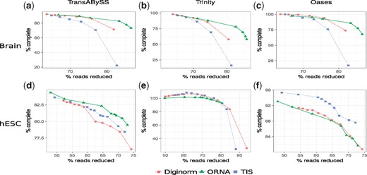
Comparison of assemblies generated from ORNA, Diginorm and TIS reduced datasets. Each point on a line corresponds to a different parametrization of the algorithms. The amount of data reduction (x-axis) is compared against the assembly performance measured as % of complete (y-axis, see text). (a) and (d) Represent TransABySS assemblies (k = 21) applied on normalized brain and hESC data, respectively. (b) and (e) Represent Trinity assemblies (k = 25) and (c) and (f) represent Oases multi-kmer assemblies applied on normalized brain and hESC data, respectively

For evaluating the PE mode, ORNA was run with k-mer value of 22 on the PE brain dataset and was compared against the PE mode of TIS and Diginorm (Supplementary Table S2). Normalized datasets were then assembled using TransABySS with k-mer size 21. A similar trend to the single-end mode was observed (Supplementary Fig. S4). At a higher percentage of reduction, the assembly performance of TIS and Diginorm normalized data degraded faster than the performance of ORNA normalized data.

Comparison of resource requirements. ORNA stores k-mers in bloom filters (Salikhov et al., 2014; implemented in the GATB library) making it runtime and memory efficient. Table 2 shows the comparison of memory and runtime required by ORNA against those required by Diginorm and TIS for brain, hESC and the combined dataset (see Methods) with k-mer value 22. For the calculations, normalized datasets were chosen to have similar read counts. ORNA and TIS were also run using one and 10 threads each. Diginorm is not parallelized. All the algorithms were run on a machine with 16 GB register memory (RDIMM) and 1.5 TB RAM. It can be observed that ORNA generally consumes less than half the memory and runtime required by TIS for a similar percentage of reduction. This is true for both the single and multi-threaded versions. A nice property of Diginorm, is that the user can set the memory used by tuning the number of hashes and the size of each hash. A low number of hashes would reduce the runtime of Diginorm but increases the probability of false positive k-mers. A higher number of hashes reduce false positives but Diginorm takes longer. In this work, two different parametrizations, denoted as Diginorm^a and ^b, were considered. The first uses less and the second a similar amount of memory compared to ORNA. In both cases, ORNA has an advantage of runtime over Diginorm. Similar results were also observed for PE mode (Supplementary Table S4). While Diginorm’s memory can be flexibly set, we note that ORNA uses much less space than the assembly of the reduced dataset itself, therefore not restraining the workflow.

Table 2.

Runtime (in minutes) and memory (in GB) required by different normalization algorithms

Method	Brain (147 M–20.1 GB)			hESC (142 M–13.2 GB)			Combined (883 M–98.1 GB)
	%Reduced	Time [min]	Mem [GB]	%Reduced	Time[min]	Mem [GB]	%Reduced	Time[min]	Mem [GB]
ORNA	83.3	104 (41)	6.62 (5.57)	63.90	58 (21)	6.16 (6.11)	81.4	740 (314)	32.9 (33.01)
Diginorma	81.86	110	3.13	61.63	115	3.13	80.37	760	12.51
Diginormb	81.51	135	6.26	62.59	126	6.26	79.31	2158	34.3
TIS	83.92	160 (95)	20.39 (20.19)	62.16	145 (127)	13.54 (13.53)	82.04	1859 (783)	95.19 (96.09)

Notes: Time and memory as obtained by running with 10 threads are shown in brackets (if possible). Note that the memory of Diginorm can be set by the user. For comparison it is set such that it uses less or similar memory than ORNA denoted as Diginorm ^a and ^b, respectively. The percent of reads reduced by each method (% reduced) is shown in the first column for each dataset. The total number of reads (in millions) and the file size (in GB) of the original dataset is shown in brackets next to the dataset.

3.2 Combined error correction and normalization generates fast and accurate de novo assemblies

As ORNA retains all the k-mers from the original dataset, useless or erroneous k-mers are also retained. As Figure 4a shows, running ORNA on the corrected brain data reduces more reads compared to the uncorrected data and leads to an improvement in assembly performance, tested with Oases multi-k assemblies. For a similar % of reduction, the EC data leads to more full length assemblies. This suggests that it is important to error correct the data before normalization with ORNA.

Fig. 4.

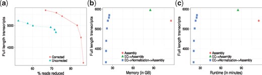
Oases assembly performance using ORNA on the brain dataset. (a) ORNA normalization on uncorrected (dashed line) and error corrected (EC, solid line) data. The points on the curve represent how many full length transcripts (y-axis) have been assembled at a particular percent of reduction (x-axis). (b) Analysis of memory required (x-axis) by different assembly strategies namely–assembling uncorrected data (cross), assembling EC data (circle) and assembling EC and normalized data (rectangle). (c) Analysis of runtime (x-axis) required by the three strategies

For a given dataset, assembly can be performed on–(i) the original dataset, (ii) EC dataset, (iii) EC and normalized dataset. Figure 4b and c show the maximum memory and runtimes required by applying these different strategies to the brain dataset. As seen from Figure 4b, memory required to assemble the uncorrected brain dataset is quite high. This is because of erroneous k-mers that complicate the graph as well as the high redundancy in the dataset. Memory is reduced by nearly 20% after error correction. It is further reduced by nearly 80% when the EC data is normalized using ORNA and then assembled.

Runtime required to assemble a high coverage dataset is generally high (Fig. 4c). Error correcting the data improves the assembly but increases the runtime of the entire process. Normalizing EC data and then assembling it reduces the runtime by nearly 40% but still generates a high number of full length transcripts. Interestingly, for three ORNA parameters (b = 1.3, 1.5, 1.7) the assembly quality (in terms of number of full length transcripts) is better than assembly of the uncorrected data with much lower time and memory consumption. For more stringent parameters (⁠$b>$1.7) the quality degrades due to a high % of reduction. Note that it is likely that similar conclusions could be made using Diginorm or TIS as normalization method. Thus in combination, error correction and normalization of RNA-seq data can be considered as potent pre-processing steps to an assembly procedure.

3.3 Finding novel transcripts by joint normalization of large datasets

Another important application of RNA-seq assembly methods is to find novel, unknown transcripts in well-annotated genomes by analyzing dozens of datasets of specialized tissues, e.g. in cancer (White et al., 2014). The common routine in these works is to assemble each RNA-seq dataset individually. It can be argued, that instead of running the assemblies on the individual datasets, a combined dataset may allow to assemble transcripts that are not well covered in an individual dataset. But combining datasets increases the size of the dataset and thereby increases the resource requirements. Hence, the dataset has to be normalized first to remove redundancy. In this work, five diverse RNA-seq datasets were concatenated to form a combined dataset of 883 M reads. The combined dataset was assembled using TransABySS and a total of 5201 full length hits were obtained. Assembling the combined dataset required 357 GB of RAM and took 73 h to produce the final assembly. ORNA reduced the combined dataset to 163 M reads. Assembling the reduced dataset using TransABySS resulted in 4821 full length hits. A memory of 28 GB and a runtime of 25 h were required to assemble the reduced dataset.

The assembly generated from the reduced combined dataset was then used to obtain missed transcripts. Note that missed transcripts refer to the transcripts, which were only assembled from the combined reduced dataset and not the individual datasets, see Materials and methods Section. The missed transcripts were aligned against the genome and compared against Ensembl annotations to estimate the number of full-length transcripts that have been missed by the individual assemblies. The biotypes of the full-length transcripts were obtained from Ensembl and GENCODE. Overall 381 missing protein coding transcripts were obtained by assembling the combined datasets. Along with these, 22 long non-coding RNAs, 49 non-coding RNAs and 15 pseudogenes are also part of the missed transcripts. Similar results may be obtained with Diginorm or TIS, albeit only ORNA guarantees that no k-mer information is lost.

4 Discussion and conclusion

This work presents ORNA, a SMC optimization-based algorithm to reduce the redundancy in NGS data without losing any k-mer information important for DBGs. This is done by approximating the minimal number of reads required to retain all k-mers from the original dataset. By generating k-mer specific normalization weights, ORNA is able to retain the relative abundance difference between k-mers. This is important as various assemblers for non-uniform sequencing datasets use the abundance information to resolve complex graph sub-structures. ORNA, when tested on multiple datasets, is able to reduce up to 85% of the data and still able to maintain nearly 80% of useful transcripts.

The performance of ORNA was compared against two well established normalization algorithms–Diginorm and TIS normalization. Brain and hESC datasets reduced by these three algorithms were assembled using Oases, Trinity and TransABySS. The assembled transcripts were then evaluated using the REF-EVAL component of DETONATE. In general, assemblies generated from ORNA reduced datasets were having a similar or higher F1 score as compared to Diginorm and TIS reduced datasets. Concerning the amount of full-length assemblies, ORNA reduced datasets performed better than Diginorm and TIS reduced datasets on the brain data. For hESC data, the results were heterogeneous and depended on the assembler used. This behaviour was corroborated by the F1-score results for hESC data, where the nucleotide recall of Oases assemblies from ORNA reduced datasets were smaller compared to TIS and Diginorm. There might be several factors such as the distribution of kmers in the original dataset and the heuristic approaches used by the assemblers, which might explain these variations.

As throwing away data may show unexpected results, the same parameter of a normalization algorithm may lead to variable reduction values for different datasets. Currently, there is no clear way how to set these parameters given the data at hand. A recent work has shown how to optimize k-mer values for multi-kmer assembly (Durai and Schulz, 2016). Such an automatic selection procedure for the k-mer value used for normalization would be worthwhile as well.

Despite the previously shown advantage of assembly runtime and memory after read normalization, it was investigated how combining and normalizing many datasets can generate novel transcripts. Intuitively, low-coverage transcripts will never be assembled or even detected in a single sequencing run. However, once many of these experiments are combined the coverage may be sufficient for assembly. It was illustrated that combining five diverse datasets led to the full-length assembly of more than 400 transcripts that would have been missed otherwise. This suggests that novelty detection approaches, e.g. in cancer samples could use that strategy to combine and normalize all datasets.

Variation in the performance of ORNA, when different measures are used, underlines the fact that ORNA is a heuristic algorithm that can be tuned further for better results. At the moment, ORNA works best when the input data is EC. As it focuses on retaining all the k-mers from the original dataset, any erroneous k-mer which escapes the filter of error correction is retained. Zhang et al., 2015 observed that error correction before applying Diginorm to a dataset improved assembly performance. An extra filtering criteria like the quality score can also be incorporated to remove erroneous k-mers or to improve the ordering of the reads.

As a conclusion, this work suggests a SMC based approach for removing read redundancy in large datasets and shows an improvement over the current normalization methods, in particular for single k-mer transcriptome assemblies. Although ORNA was only applied on RNA-seq data, the algorithm can also be applied for other non-uniform datasets from metagenomics or single-cell sequencing. The software is freely available at https://github.com/SchulzLab/ORNA.

Funding

This work was supported by the Cluster of Excellence on Multi-modal Computing and Interaction (EXC284) of the German National Science Foundation (DFG); and International Max Planck Research School for Computer Science, Saarbrücken.

Conflict of Interest: none declared.