


Abstract
RNA-binding proteins (RBPs) take over 5–10% of the eukaryotic proteome and play key roles in many biological processes, e.g. gene regulation. Experimental detection of RBP binding sites is still time-intensive and high-costly. Instead, computational prediction of the RBP binding sites using patterns learned from existing annotation knowledge is a fast approach. From the biological point of view, the local structure context derived from local sequences will be recognized by specific RBPs. However, in computational modeling using deep learning, to our best knowledge, only global representations of entire RNA sequences are employed. So far, the local sequence information is ignored in the deep model construction process.
In this study, we present a computational method iDeepE to predict RNA–protein binding sites from RNA sequences by combining global and local convolutional neural networks (CNNs). For the global CNN, we pad the RNA sequences into the same length. For the local CNN, we split a RNA sequence into multiple overlapping fixed-length subsequences, where each subsequence is a signal channel of the whole sequence. Next, we train deep CNNs for multiple subsequences and the padded sequences to learn high-level features, respectively. Finally, the outputs from local and global CNNs are combined to improve the prediction. iDeepE demonstrates a better performance over state-of-the-art methods on two large-scale datasets derived from CLIP-seq. We also find that the local CNN runs 1.8 times faster than the global CNN with comparable performance when using GPUs. Our results show that iDeepE has captured experimentally verified binding motifs.
Supplementary data are available at Bioinformatics online.
1 Introduction
RNA-binding proteins (RBPs) are highly involved in many biological processes, e.g. gene regulation (Gerstberger et al., 2014) and mRNA localization (Dictenberg et al., 2008), and they take over 5–10% of the eukaryotic proteome (Castello et al., 2012). Some mutations of RBPs might cause diseases. For example, the mutations in RBP FUS and TDP-43 can cause amyotrophic lateral sclerosis (Mackenzie et al., 2010). Thus, decoding the overview of RBP binding sites can give deeper insights into many biological mechanisms (Glisovic et al., 2008).
With the high-throughput technologies developing, e.g. CLIP-seq (Anders et al., 2012; Ferre et al., 2016; Ray et al., 2013), a huge volume of experimentally verified RBP binding sites are generated. However, they are time-consuming and high-costly. Fortunately, these experimental data can serve as training data for machine learning models to learn binding patterns of RBPs. Many computational approaches have been proposed to predict RBP binding sites (Corrado et al., 2016; Kazan et al., 2010; Maticzka et al., 2014; Strazar et al., 2016). For example, RNAContext is designed to identify RBP-specific sequence and structural preferences (Kazan et al., 2010). GraphProt encodes the sequence and structure of RNAs using graph encoding, which are further fed into support vector machines (SVMs) to classify bound sites from unbound sites (Maticzka et al., 2014). RNAcommender applies a recommender system to suggest binding targets for RBPs by propagating the protein domain composition and the predicted RNA secondary structures (Corrado et al., 2016). The iONMF integrates multiple sources of data, e.g. sequences, structures, gene types and clip-cobinding, using orthogonal matrix factorization (Strazar et al., 2016).
Recently, deep learning (Hinton and Salakhutdinov, 2006; LeCun et al., 2015) based methods have attracted huge attention for predicting protein-binding RNAs/DNAs (Alipanahi et al., 2015; Pan et al., 2016; Pan and Shen, 2017; Zhang et al., 2016), especially convolutional neural networks (CNNs) (Lecun et al., 1998) based methods. These methods not only outperform other existing methods in terms of prediction accuracy, but also can easily extract binding motifs directly from the learned parameters of CNNs. For example, DeepBind trains a CNN model to identify the binding preference of RNA- and DNA-binding proteins (Alipanahi et al., 2015). DeepSea also trains a CNN model to predict the chromatin effects of sequence alteration from sequences (Zhou and Troyanskaya, 2015). Considering the complementarity of multiple sources of data, e.g. sequence, structure and genomic context, our previous iDeep model integrates deep belief networks (DBNs) (Hinton and Salakhutdinov, 2006) and a CNN, resulting in an improved performance (Pan and Shen, 2017). Different from DeepBind, iDeepS takes structures into consideration for RBP binding specificity (Pan et al., 2017), and it trains two individual CNNs and a long short term memory network (LSTM) (Hochreiter and Schmidhuber, 1997) for sequences and structures to capture binding sequence and structure motifs of RBPs. Since the CNN-based methods require input sequences with the same length, to handle the sequence with variable length, one solution is padding all sequences according to the longest sequence in training set.
Although, several conventional machine learning-based methods, such as Global Score (Cirillo et al., 2017), omiXcore (Armaos et al., 2017) and RPI-Bind (Luo et al., 2017), employ local features of RNAs and proteins to predict RNA–protein interaction pairs, almost all previous deep learning based RBP-specific approaches employ only entire sequences, and the local sequences are not taken into account so far during model training. However, the RNA targets of an RBP generally share common local sequences, and are also mediated by structure context (Lange et al., 2012). Structural effects are limited to local domain that has impact on regional RNA recognition motifs (Liu et al., 2017). Local structures are derived from local sequences, thus those local sequences play important roles in RNA–protein interactions (Grover et al., 2011; Tafer et al., 2008). To integrate the local sequence information, we first split sequences to multiple overlapping fixed-length subsequences, each subsequence is considered as a channel like RGB channels of images. On the other hand, an entire RNA sequence contains an overview of the buried information without breaking some crucial information for RBP interactions.
In this study, we present a new computational method iDeepE for predicting RBP binding sites and motifs. It trains a local multi-channel CNN and a global CNN for multiple local subsequences and entire sequences, respectively. Considering that the ensemble of CNNs are known to be more robust and accurate than individual CNNs (Hinton et al., 2015; Pan et al., 2011), we integrate the local and global CNNs as the final model to improve the performance. iDeepE also supports GPU acceleration. Furthermore, we designed different network architectures based on CNNs, e.g. CNNs, CNN-LSTM and Deep Residual Net (ResNet) (He et al., 2016a,b), and compared them with other state-of-the-methods for predicting RBP binding sites on RNAs. In addition, through evaluating the extracted binding sequence motifs from iDeepE against experimentally verified binding motifs, we demonstrate that iDeepE can capture binding motifs.
2 Materials and methods
In this study, we present a deep learning-based approach, iDeepE (Fig. 1, Supplementary Algorithm 1), to predict the RBP binding sites by integrating a local multi-channel CNN and a global CNN. We first collect two large-scale RBP binding sites datasets, which are used to train and evaluate the iDeepE. Next, we give the technical details about different deep neural networks, including CNN, LSTM, ResNet and their combinations in details.
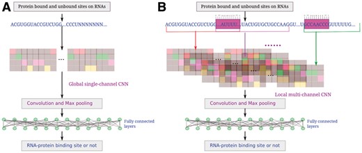
The flowchart of iDeepE, it trains one model per RBP. (A) It pads the RNA sequences to the maximum length in training sequences, and they are converted into one-hot matrix, which are fed into a global CNN. (B) It first breaks each RNA sequence into multiple overlapping fixed-length subsequences, each subsequence is a channel like RGB channel in images. Next these subsequences are encoded in one-hot matrix (The gray is 0 and other colors are 1), which are further inputted into a local multi-channel CNN. Finally, the predictions are combined to yield the final predictions by averaging the output probabilities from the global CNN (A) and local CNN (B)
2.1 Datasets and data preprocessing
The iDeepE model is evaluated on two large-scale datasets derived from CLIP-seq: RBP-24 and RBP-47.
RBP-24: Here, the training and testing datasets of RBP binding sites are downloaded from the website of GraphProt (http://www.bioinf.uni-freiburg.de/Software/GraphProt). This dataset is also used by deepnet-rbp (Zhang et al., 2016). It covers 24 experiments of 21 RBPs. For each experiment, the positive sites are subsequences anchored at the peak center derived from CLIP-seq processed in doRiNA (Anders et al., 2012), the negative sites are the regions with no supportive evidence of being binding sites. A number of training samples are listed in Supplementary Table S1. For independent testing set, most RBPs have 500 positives and 500 negatives, which are original GraphProt's testing set.
RBP-47: We also collect the datasets from RNAcommender (Corrado et al., 2016), which includes a total of 502 178 binding sites for 67 RBPs from CLIP-seq, but with different number of binding sites for individual RBPs (Supplementary Table S2). We only keep those RBPs with the number of positive UTR sequences greater than 2000. It is because deep learning based methods cannot converge on a too small training set. In the end, we obtain the remaining 47 RBPs for following experiments. To train a model for each RBP, we also generate the same number of negative sequences by randomly selecting the UTRs not interacting with this RBP. Furthermore, we also create an non-redundant RBP-47 dataset, in which RNA sequences in testing set with sequence similarity greater than 80% to any sequences in training set were excluded by using cd-hit-est in CD-HIT tool (Huang et al., 2010). 80% is the minimum cutoff value of cd-hit-est, for lower cutoff, we use cd-hit to reduce sequence redundancy.
In summary, RBP-24 is a subsequence-level dataset, and RBP-47 is a UTR-level dataset. For these two datasets, the positive sets are both derived from CLIP-seq, but the negative sets are generated in different strategies. The negative set of each RBP in RBP-24 is produced by moving the positive binding sites to random regions in the same gene. However, the negative set of each RBP in RBP-47 consists of the UTRs not interacting with this RBP.
We use different strategies to construct negative sequences of RBP24 and RBP47 due to the followings: (i) We want to align and compare with the original methods of GraphProt and RNAcommender, and the two methods construct negative sequences using different ways. (ii) Negative sequences of RBP-24 are subsequences of other non-bound region from the same gene of positive sequences, while the negative sequences of RBP-47 are UTRs from different genes. As shown in iONMF (Strazar et al., 2016), region types also have important discriminate ability for RBP binding sites. Thus, we cannot simply use other regions (e.g. exon, intron, etc.) of the same gene as negative sequences for RBP-47. We also use CD-HIT to exclude those redundant sequences in testing set with sequence similarity over 80% to any sequences in training set.
2.2 Sequence encoding
The CNN model requires that the inputs have fixed lengths, whereas different RNA sequences vary significantly on their lengths. To solve this problem, we do the following preprocessing for the input RNA sequences:
For the global CNN module, all the sequences are padded into the maximum length according to the predefined longest sequence in the training set.
For the local CNN, we first break the RNA sequence of length L into multiple subsequences with window size W, each subsequence is considered as a channel. The number of subsequences with overlapped shift S in the whole sequence is therefore (L—W)/(W—S). Here we also calculated the maximum number of channels C according to the maximum length in training sequences. If the number of channels for one sequence is smaller than C, then it is extended by channels derived from sequences with all nucleotide Ns to the C.
2.3 Convolutional neural network, long short term memory network and Residual Net
Long short term memory network (LSTM) (Hochreiter and Schmidhuber, 1997) is a widely used recurrent neural networks, it is capable of learning long-term dependencies to improve prediction performance. A LSTM consists of a forget gate layer, an input gate layer and an output layer. LSTM first decides which information should be excluded by a forget gate layer according to previous inputs. Then an input gate layer determines which information should be kept for next layer, and update the current state value. Finally, an output gate layer is used to decide what parts of state value should be outputted.
Bidirectional LSTM (BLSTM) is used to learn two directional dependency, which sweeps from both left to right and right to left, and the outputs of individual directions are concatenated. For CNN-LSTM, the learned feature maps from CNNs are subsequently fed into a bidirectional LSTM to learn long range dependencies between those feature maps.
2.4 Identifying the binding sequence motifs
We investigate convolution filters of the global CNN integrated in iDeepE. The learned parameters of these convolve filters are converted into position weight matrices (PWM) using the same strategy in DeepBind and Basset (Alipanahi et al., 2015; Kelley et al., 2016). For each sequence in a set of sequences and filter of width , k-mer sequence is selected, if the activation of filter at position is greater than 0.5 maximum activation of this filter across this set of sequences. Those selected k-mer sequences are aligned using WebLogo (Crooks et al., 2004) to get sequence motifs.
To verify the detected sequence motifs, we align them against experimentally discovered motifs from CISBP-RNA (Ray et al., 2013) using the TOMTOM (Gupta et al., 2007) algorithm with P-value <0.05. In addition, we also evaluate the motif enrichment score using AME (Buske et al., 2010) in the MEME suite (Bailey et al., 2009). It estimates the enrichment scores by scanning the predicted motifs against the input sequences and corresponding shuffled sequences.
All the detected motifs for individual RBPs in RBP-24 dataset are available at https://github.com/xypan1232/iDeepE/tree/master/motif, which gives the learned filter heatmaps, WebLogo motifs, enrichment scores and the outputs from TOMTOM. In addition, all enrichment analysis of all motifs for individual RBPs are also given at the same site. We also calculate the motif frequencies in binding and non-binding sites using FIMO in MEME, respectively.
2.5 Models and baselines
Many computational methods have been developed for predicting RBP binding sites from sequences alone. In this study, we evaluate our method iDeepE and its eight variants against three state-of-the-art methods, and the network architectures are shown in Supplementary Material.
iDeepE-L: It uses two-layer local multi-channel CNNs (convolution, ReLU and max pooling) to convolve the multiple subsequences of RNA sequences in parallel, then the feature maps are further fed into two fully connected layers.
iDeepE-G: It uses two-layer global 1-channel CNNs for padded RNA sequences, where all the sequences are padded into the same length, then the feature maps from 1-channel CNN are inputted into two fully connected layers. It uses the same technique as DeepBind.
iDeepE: It averages the output probabilities from iDeepE-L and iDeepE-G as the final predictions.
CNN-LSTM-L: It is similar to iDeepE-L with an additional two-layer bidirectional LSTM layer before the two fully connected layers.
CNN-LSTM-G: It is similar to iDeepE-G with an additional two-layer bidirectional LSTM layer before the two fully connected layers.
CNN-LSTM-E: It is the ensembling of CNN-LSTM-L and CNN-LSTM-G.
ResNet-L: It uses 21-layer local multi-channel CNNs, and insert shortcut connections between each two CNNs, which turn the network into its counterpart residual.
ResNet-G: It uses 21-layer global 1-channel CNNs, and insert shortcut connections between each two CNNs, which turn the network into its counterpart residual.
ResNet-E: It is the ensembling of ResNet-L and ResNet-G.
GraphProt (Maticzka et al., 2014): It represents the RNA sequences and structures in a high dimensional graph features, which are further fed into support vector machine to classify bound sites from unbound sites.
deepnet-rbp (Zhang et al., 2016): It trains a deep belief network to predict RBP binding sites using the k-mer frequency features of sequences and structures.
Pse-SVM: we also developed another method using pseudo components generated by Pse-In-One(Liu et al., 2015a,b) with parameters ‘-lamda 2 –w 0.05’as input features, which are fed into a support vector machine (SVM) to classify bound sites from unbound sites. We use grid search to find the optimum parameters of SVMs for each RBP. Both the SVM and grid search are from scikit-learn (Pedregosa et al., 2011), and the values to be searched for SVM parameter C is [1, 5, 10], and gamma is [0.01, 0.1, 1].
In this study, considering the binding specificity of RBPs, we train RBP-specific model, where each model is trained on RNA sequences for each RBP. Thus we only choose sequence-based methods GraphProt, deepnet-rbp, Pse-SVM and DeepBind as our baseline methods. Here, iDeep and iDeepS are excluded for comparison. It is because of the following: (i) iDeep requires other sources of features, like region type and clip-cobinding. In addition, iDeep currently can only handle fixed-length sequences. (ii) iDeepS cannot handle long RNA sequences well, it is because predicting RNA structures from sequences is computationally intensive, especially for long RNA sequences in RBP-47. In this study, we use one-hot encoding to represent RNA sequences, we also compare iDeepE with another method Pse-SVM that uses k-tuple nucleotide composition.
There also exist some non-RBP-specific methods that train a mixed model (Armaos et al., 2017; Cirillo et al., 2017; Kumar et al., 2008) on RNA and protein sequences together without considering the binding specificities of RBPs. To demonstrate that RBP-specific model yield better performance, we also evaluate non-RBP-specific omiXcore (Armaos et al., 2017) on testing set of RBP-24.
2.6 Experimental details
To create local subsequences for local CNNs from entire sequences, we use grid search to select optimum parameters window size W and shift size S with other hyper parameters of CNNs. We configure the maximum length of sequences L = 501 and L =2695 for RBP-24 and RBP-47, respectively. It is because the sequences in RBP-47 are much longer than RBP-24. The value L is chosen to ascertain that over 90% of sequences in train set are shorter than L. For sequences longer than L, they will be truncated to length L.
We implement the iDeepE using PyTorch 0.1.11 (http://pytorch.org/), it supports strong GPU acceleration. We set the number of epochs to 50, and the batch size to 100, and Adam is used to minimize binary cross-entropy loss. The parameter number of filters is set to 16 (Alipanahi et al., 2015). The length of verified motifs in CISBP-RNA database is 7 (Ray et al., 2013), as suggested by DeepBind that the parameter kernel size should be 1.5 times the length of verified motifs, and hence the kernel size is 10. The initial weights and bias use default setting in PyTorch. When converting them to binding motifs, we only use the previous 7 bits to match the verified motifs in CISBP-RNA database. In addition, we also employ multiple techniques to prevent or reduce over-fitting, e.g. batch normalization and dropout (Srivastava et al., 2014).
We run our experiments on a Ubuntu server with TITAN X GPU with memory 12 GB. We use the area under the receiver operating characteristic curve (AUC) to measure the performance of different methods.
3 Results
In this section, we first compare iDeepE with its variants and other state-of-the-art methods, then we investigate the difference between local CNNs and global CNNs. Furthermore, we infer the binding motifs from the parameters of CNNs, and evaluate the identified motifs against experimentally verified motifs in CISBP-RNA. Additionally, we also evaluate the iDeepE on RBP-47 dataset and cross-dataset performance between RBP-24 and RBP-47.
3.1 Parameter optimization
To investigate the impact of parameters on the performance of iDeepE, we use 90% of original training set from RBP-24 as training set, and the remaining 10% as validation set. We apply grid search to find the best parameters for iDeepE, including hyperparameters of CNNs (dropout probability D with values [0.25, 0.5], learning rate LR with values [0.001, 0.0001] and regularization weight_decay WD with values [0.01, 0.001, 0.0001]), windows size W with values [81, 101, 151] and overlapped shift size S with values [20, 30, 50] for local CNNs. In total, we evaluate the performance (mean AUCs across 24 RBPs are shown in Supplementary Table S3) of iDeepE for 108 combinations of these 5 parameters. We yield the best mean AUC 0.934 when D = 0.25, LR = 0.001, WD = 0.0001, W = 151 and S = 30. Considering that the larger the window size W is, the less the number of subsequences is, thus the more time-consuming iDeepE is, we choose W = 101, which is also used in previous studies (Pan and Shen, 2017; Strazar et al., 2016). Thus, when we fixed the W = 101, iDeepE yields the best mean AUC 0.931 when D = 0.25, LR = 0.001, WD = 0.0001 and S = 50. In addition, we plot figures of performance change related to the five parameters individually (Supplementary Fig. S1). In each figure, the x-axis corresponds to the same values of other 4 parameters. When measuring their impact individually, we can see that smaller dropout D, larger window size W and smaller WD can yield better performance, learning rate LR and shift size S have no obvious impact on performance. Considering it is very time-intensive to optimize these parameters, for RBP-47 dataset, we use S = 20 to make less overlap between windows for long RNA sequences in RBP-47, LR = 0.0001, and the same values for other 3 parameters.
3.2 The performance of iDeepE on RBP-24
As shown in Table 1, iDeepE yields the best average AUC of 0.931 across 24 experiments, which is better than 0.887 of GraphProt, 0.912 of CNN-LSTM-E, 0.919 of ResNet-E, 0.778 of Pse-SVM and 0.902 of deepnet-rbp. Of the 3 fully sequence-based predictors using local or global CNNs, all 3 predictors perform better than sequence-structure-profile based methods GraphProt and deepnet-rbp. According to the experiments, ResNet-E yields worse performance than iDeepE on RBPs (e.g. ALKBH5 and C17ORF85) and the potential reason is that it is constructed with a small number of training sequences. We also found that the tested Pse-SVM performs worse than other approaches. The potential reason is that the parameters of Pse-In-One need be further tuned to generate better pseudo component features instead of using default parameters. The developed iDeepE model yields the best AUC on 17 experiments among the 6 predictors, followed by deepnet-rbp with 6 experiments. Compared to DBN-based deepnet-rbp, iDeepE can achieve an obvious improvement for some proteins, e.g. ZC3H7B, which is an increase by 13.9% from 0.796 of deepnet-rbp to 0.907 of iDeepE. For the same protein ZC3H7B, iDeepE also performs better than the AUC 0.820 of GraphProt, and iDeepE increase the AUC 0.765 of GraphProt for RBP Ago2 to 0.884, which is an increase by 15.5%. In addition, we also run iDeepE on non-redundant RBP-24 dataset, in which RNA sequences in testing set have sequence similarity 80, 70 and 60% smaller than any sequences in training set, respectively. iDeepE achieves average AUCs of 0.928, 0.920 and 0.918 (Supplementary Fig. S2), which are a little lower than the AUC 0.931 on the original set.
The performance of iDeepE and other baseline methods across 24 experiments on RBP-24 dataset
| RBP | iDeepE | CNN-LSTM-E | ResNet-E | Pse-SVM | GraphProt | Deepnet-rbp |
|---|---|---|---|---|---|---|
| ALKBH5 | 0.758 | 0.653 | 0.656 | 0.648 | 0.680 | 0.714 |
| C17ORF85 | 0.830 | 0.822 | 0.756 | 0.734 | 0.800 | 0.820 |
| C22ORF28 | 0.837 | 0.801 | 0.829 | 0.764 | 0.751 | 0.792 |
| CAPRIN1 | 0.893 | 0.871 | 0.891 | 0.728 | 0.855 | 0.834 |
| Ago2 | 0.884 | 0.851 | 0.854 | 0.746 | 0.765 | 0.809 |
| ELAVL1H | 0.979 | 0.975 | 0.975 | 0.816 | 0.955 | 0.966 |
| SFRS1 | 0.946 | 0.929 | 0.945 | 0.746 | 0.898 | 0.931 |
| HNRNPC | 0.976 | 0.973 | 0.975 | 0.824 | 0.952 | 0.962 |
| TDP43 | 0.945 | 0.928 | 0.937 | 0.840 | 0.874 | 0.876 |
| TIA1 | 0.937 | 0.911 | 0.929 | 0.784 | 0.861 | 0.891 |
| TIAL1 | 0.934 | 0.901 | 0.930 | 0.724 | 0.833 | 0.870 |
| Ago1-4 | 0.915 | 0.873 | 0.911 | 0.728 | 0.895 | 0.881 |
| ELAVL1B | 0.971 | 0.963 | 0.970 | 0.837 | 0.935 | 0.961 |
| ELAVL1A | 0.964 | 0.962 | 0.961 | 0.830 | 0.959 | 0.966 |
| EWSR1 | 0.969 | 0.965 | 0.967 | 0.753 | 0.935 | 0.966 |
| FUS | 0.985 | 0.980 | 0.977 | 0.762 | 0.968 | 0.980 |
| ELAVL1C | 0.988 | 0.986 | 0.988 | 0.853 | 0.991 | 0.994 |
| IGF2BP1-3 | 0.947 | 0.940 | 0.952 | 0.753 | 0.889 | 0.879 |
| MOV10 | 0.916 | 0.899 | 0.911 | 0.783 | 0.863 | 0.854 |
| PUM2 | 0.967 | 0.963 | 0.965 | 0.840 | 0.954 | 0.971 |
| QKI | 0.970 | 0.966 | 0.969 | 0.809 | 0.957 | 0.983 |
| TAF15 | 0.976 | 0.974 | 0.971 | 0.769 | 0.970 | 0.983 |
| PTB | 0.944 | 0.929 | 0.943 | 0.867 | 0.937 | 0.983 |
| ZC3H7B | 0.907 | 0.879 | 0.906 | 0.743 | 0.820 | 0.796 |
| Mean | 0.931 | 0.912 | 0.919 | 0.778 | 0.887 | 0.902 |
Note: The AUCs for GraphProt and deepnet-rbp are taken from original papers. The boldface indicates this AUC is the best among compared methods.
It needs to be pointed out that iDeepE performs worse on RBPs with a small training set, e.g. ALKBH5 with 2410 training samples and C17ORF85 with 3709 training samples (Supplementary Table S1). It is because CNN-based methods in general require more data to yield a better model. iDeepE achieves better performance than its base predictors iDeepE-G and iDeepE-L, indicating that the two predictors can complement with each other. The ensemble predictor of local and global CNNs outperform other two ensemble predictors CNN-LSTM-E and ResNet-E that have more complex network architectures.
We also compare iDeepE with non-RBP-specific method omiXcore with protein and RNA sequences as inputs. We use omiXcore to estimate binding scores between each RBP sequence and its testing RNA sequences in RBP-24. Then based on these scores, we calculate the AUC for each RBP. Here, we evaluate omiXcore on 17 RBPs, and omiXcore yields an average AUC 0.54 (Supplementary Fig. S3), which is worse than iDeepE. The results indicate that RBP-specific model can yield better performance than non-RBP-specific method. The reason is that different RBPs show different binding specificities, which is ignored by the non-RBP-specific method omiXcore.
3.3 Comparing local CNNs with global CNNs on RBP-24
As indicated in Figure 2A, different models' performances vary on different datasets, and no single predictor can beat others on all datasets. The six predictors iDeepE-L, iDeepE-G (DeepBind), CNN-LSTM-L, CNN-LSTM-G, ResNet-L and ResNet-G yield the average AUCs of 0.909, 0.925, 0.898, 0.900, 0.902 and 0.916 across 24 experiments, respectively. The results show that for most RBPs, ResNet performs similar to others, but ResNet performs worse than others on RBPs with small number of training set (e.g. ALKBH5). It might be because that more complex models require more training data, although ResNet has been demonstrated that it is powerful in image recognition. The deeper the model is, the more number of training samples it requires.
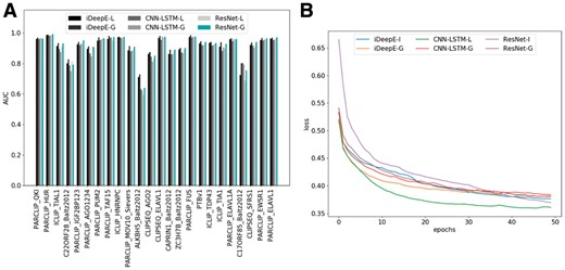
Comparing local CNNs with global CNNs on RBP-24 dataset. (A) The AUCs of local and global CNNs integrated in iDeepE, CNN-LSTM and ResNet across 24 experiments in RBP-24. All the models are ran on the same training and testing datasets. (B) The averaging training loss across 24 experiments in RBBP-24 changes with the number of epochs for deep networks using local and global CNNs
Furthermore, we also show the average training loss change for 24 experiments with the number of epochs (Fig. 2B). The results show that the local CNNs converge to lower training loss than their corresponding global ones, but their performance are worse. And the training process converges after about 50 epochs. The CNN-LSTM-L yields lower loss than iDeepE-L and ResNet-L, but it performs worse on independent testing set (Fig. 2A). The results implicate that CNN-LSTM-L suffers to over-fitting. Similarly, ResNet-G has lower training loss, but yields lower performance than its peer iDeepE-G. The results demonstrate that using too much deeper networks for RNA sequences cannot guarantee better models, which is different from the huge success on images. From Figure 2B, we also can see that iDeepE-L and CNN-LSTM-L almost have the same training loss and converging to the same loss consistently. The local CNN converges slower than the corresponding global CNN.
We also record the total time cost of individual models on our training data (Table 2). The results indicate that the local multi-channel CNN performs faster than the global CNN. iDeepE-L is over 1.8 times faster than iDeepE-G, and CNN-LSTM-L is nearly 1.5 times faster than CNN-LSTM-G. We can obviously see that ResNet runs much slower than other models, it is because ResNet has over 5 times deeper than other models.
The total time cost of different models for training the 24 experiments in RBP-24
| Method | Time (s) |
|---|---|
| iDeepE-L | 3741.31 |
| iDeepE-G | 6963.1 |
| CNN-LSTM-L | 6129.64 |
| CNN-LSTM-G | 9783.3 |
| ResNet-L | 20 899.78 |
| ResNet-G | 29 302.88 |
| Method | Time (s) |
|---|---|
| iDeepE-L | 3741.31 |
| iDeepE-G | 6963.1 |
| CNN-LSTM-L | 6129.64 |
| CNN-LSTM-G | 9783.3 |
| ResNet-L | 20 899.78 |
| ResNet-G | 29 302.88 |
3.4 The identified binding motifs by iDeepE
One advantage of iDeepE is that it can automatically identify the binding sequence motifs from the learned parameters of CNNs. We use iDeepE to discover binding motifs for RBPs in RBP-24 dataset. Against current CISBP-RNA, there are 3 matched motifs with significant E-value cutoff 0.05 calculated using TOMTOM are showed (Fig. 3). For ELAVL1 and its family proteins, their detected motifs are consistent with known consensus U-rich motifs derived from SELEX (Gao et al., 1994). HNRNPC also demonstrates similar preference to U-rich sites (Konig et al., 2010). For the remaining three RBPs, TIA1 and TIAL1 show a preference for U-rich binding sites (Dember et al., 1996) with E-value 0.076 and 0.07, respectively. We can find a known G-rich motif with E-value 0.07 for SFSR1 (Tacke et al., 1997).
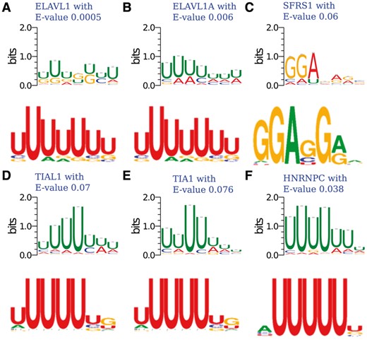
The matched motifs against experimentally verified motifs in CISBP-RNA, where the E-value is calculated by TOMTOM. In each figure (A–F), the upper figure is the detected motif by iDeepE, the below figure is the experimentally verified motifs from CISBP-RNA database
To show some meaningful motifs for those RBPS without verified motifs in current CISBP-RNA, we do the enrichment analysis for the identified motifs using AME. We show some significant motifs with support evidence from literature but absent in databases (Fig. 4). Ago2 has a binding motif identified in (Li et al., 2014) with adjusted P-value , TDP-43 shows preference for GU-rich sites with adjusted P-value 3.38 and FUS prefers to AU-rich sites with adjusted P-value 6.65(Colombrita et al., 2012). The motif of QKI closely resembles a motif reported by PAR-CLIP in (Hafner et al., 2010) with adjusted P-value . Furthermore, as shown in Supplementary Figure S4, we can see PTB has a binding motif of UC-rich sites with adjusted P-value 3(Perez et al., 1997). In addition, we identify some motifs of AU-rich sites with adjusted P-value , and for PUM2, EWSR1 and TAF15 (Hoell et al., 2011), respectively. MOV10 has preference to AC-rich sites with adjusted P-value . We also discover some novel motifs for Ago1-4, CAPRIN1 and ZC3H7B with adjusted P-value , and , respectively.
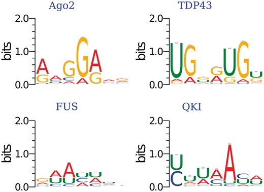
The enriched binding motifs calculated by AME. The motif P-value are calculated against shuffled sequences using AME
3.5 The performance of iDeepE on UTR-level dataset RBP-47
We further evaluate the iDeepE with local and global CNNs on a more challenging dataset RBP-47, which has more number of RBPs and UTR sequences as training samples. iDeepE, iDeepE-G, iDeepE-L and Pse-SVM yield the average AUC 0.80, 0.78, 0.75 and 0.76 across 47 RBPs, respectively. The details are shown in Supplementary Table S2. In addition, we evaluate iDeepE on stringent non-redundant dataset RBP-47, iDeepE, iDeepE-G and iDeepE-L yields the average AUCs 0.72, 0.70 and 0.69 across 47 RBPs, respectively (Supplementary Fig. S5). The performance is lower than AUCs on original RBP-47. To investigate the impact of sequence similarity on predictive performance, we further test iDeepE on datasets with similarity cutoff 0.70, 0.60 and 0.50. iDeepE yields average AUCs 0.71, 0.68 and 0.57, respectively. The reason that iDeepE perform much worse on sequences with cutoff 0.50 is that too few samples are left. The corresponding results are shown in Supplementary Table S4.
Of the 47 RBPs, 36 RBPs are evaluated by both RNAcommender and iDeepE, the AUCs are shown in Figure 5A (Supplementary Table S2). iDeepE, iDeep-G, iDeep-L, RNAcommender and Pse-SVM achieves the average AUC of 0.81, 0.79, 0.76, 0.79 and 0.77 across the 36 RBPs, respectively. The results demonstrate that fusing the local and global CNNs yields better performance. Of the 36 RBPs, iDeepE yields the best AUCs on 20 RBPs. For some RBPs, it achieves an improvement with a large margin. Take RBP STAU1 as an example, iDeepE increases the AUC 0.48 of RNAcommender to AUC 0.73 by 52%. However, for some RBPs like IGF2BP1, iDeepE performs worse than RNAcommender. In addition, the local CNN can perform better than the global CNN for some RBPs (e.g. EWSR1, PUM2, Supplementary Table S2). For example, the local CNN yields an AUC 0.83 for EWSR1, which is higher than an AUC 0.81 of the global CNN. It is worth pointing out that RNAcommender trains recommend system using Factorization Machines by automatically treating full undetected interactions as negative samples. However, iDeepE only randomly selects a subset of negative sequences. In addition, compared to RNAcommender and Pse-SVM, iDeepE can identify verified binding motifs.
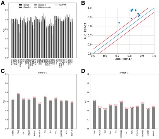
The performance of iDeepE on RBP-47 dataset and cross-dataset performance for 12 shared RBPs between RBP-47 and RBP-24 datasets. (A) The AUCs of iDeepE and other state-of-the-art methods, where the AUCs of RNAcommender directly are taken from the paper. (B) The performance of iDeepE for the shared 12 RBPs from RBP-24 and RBP-47 datasets. (C) The cross-dataset validation performance of iDeepE-1, iDeepE-1 is trained on positive and negative sets from RBP-47, and evaluated on testing sets from RBP-24. (D) The cross-dataset validation performance of iDeepE-2, iDeepE-2 is trained on positive set from RBP-47 but negative set are generated from shuffling the corresponding positive sequences, and evaluated on the testing sets from RBP-24
There are 12 RBPs shared between RBP-24 and RBP-47 dataset. As indicated in Figure 5B, the performance of RBPs in RBP-47 is worse than RBP-24. It is because of the followings: (i) The number of training samples for each RBP in RBP-47 dataset is fewer than RBP-24 (Supplementary Table S5). (ii) The negative samples in RBP-47 are generated from those UTRs still not verified in current AURA 2 database (August 5, 2015) (Dassi et al., 2014), which possibly exists some false negatives.
As shown in Supplementary Table S6, the negatives in RBP-47 is very different from negatives in RBP-24, but for most RBPs, there is big overlap between the positives in RBP-24 and RBP-47. In addition, we checked the overlap between negative samples with binding sites derived from eCLIP data (Van Nostrand et al., 2016), of the 12 shared RBPs, 5 have binding sites in eCLIP. We found that on average 47.4% of negative samples in RBP-47 overlap with binding sites derived from eCLIP data (Supplementary Table S7). The possible reason is that different experimental techniques may obtain inconsistent binding sites. However, RBP-24 generates the negative samples by moving the positive binding sites to random regions in the same gene, and it has much lower chance to be false negatives. It is because that the same CLIP-seq experiments find some regions are bound sites of a gene, and other regions of this gene are not bound sites, which have more confidence to be true negatives. However, randomly selecting negative UTRs may introduce some less-studied UTRs, whose sequencing depth are not covered at the same time by the same CLIP-seq analysis. To reduce false negatives, we may use available iCLIP (http://icount.biolab.si) and eCLIP (https://www.encodeproject.org/) (Van Nostrand et al., 2016)data collections to remove overlapped negatives with the binding sites derived from iCLIP and eCLIP.
3.6 Shuffling positive sequences as negative samples yields overestimated performance
Furthermore, we evaluate the iDeepE on training set consisting of positive sequences and shuffled positive sequences as negative samples. The results are shown in Supplementary Figure S6. iDeepE yields an average AUC of 0.92 across the 47 RBPs in RBP-47, which is possibly an overestimated performance. To prove it, we did cross-dataset performance evaluation for iDeepE trained on two different negative sets.
iDeepE-1: Train iDeepE using the positive and negative training set of 12 shared RBPs from RBP-47.
iDeepE-2: Train iDeepE using the same positive training set from RBP-47 but shuffled positive sequences as negative set for the 12 RBPs, in which we shuffle each positive sequence as a negative sample.
We evaluate the two trained iDeepE models using the same testing set of 12 shared RBPs from RBP-24. The results are shown in Figure 5C and D. The iDeepE-1 yields an average AUC 0.64 across the 12 RBPs, which is much lower than the AUC on original training set of RBP-24. The reason is that the negative sequences (moving positive sites to random region within the same gene) in RBP-24 partly overlap with the positive UTR sequences in RBP-47. However, iDeepE-2 achieves a much lower average AUC 0.49, which is close to random guessing. Besides, we also evaluate iDeepE-1 on non-redundant dataset, in which sequences in testing set with sequence similarity greater than 80% to any sequences in training set were excluded. iDeepE-1 yields the average AUC 0.62 (Supplementary Fig. S7). From the above results, we can conclude that the quality of training data plays crucial roles in model training, and the shuffled negative sequences lead to overestimated performance.
4 Discussion
In this study, the local CNN runs faster than the global CNN with comparable performance. We treat the multiple fixed subsequences with the same contribution to the final feature maps of CNNs. In future work, we can further improve it by combining multiple instance learning (MIL) framework (Minhas and Ben-Hur, 2012) with a local multi-channel CNN. It is commonly assumed that a RNA sequence not bound by a RBP is treated as a negative sequence, there is no any binding site of this RBP on this RNA. While a RNA sequence that can be bound by a RBP is considered as a positive sequence, it contains at least one binding site of this RBP. Therefore, it is fairly intuitive to consider each RNA sequence as a bag, and any subsequence of this RNA as an instance. On the other hand, iDeepE uses a simple averaging strategy to combine the local and global CNNs. In previous studies, a novel stacked ensembling strategy has been proved efficient in ncRNA–protein interaction prediction (Cao et al., 2018; Pan et al., 2016), it can be further applied to improve iDeepE’s performance.
We also demonstrate that shuffling positive sequences as negative samples will lead to overoptimistic performance when constructing training dataset. The reason is that shuffled sequences are not real sequences that can be captured by CLIP-seq. However, negative samples generated by moving the positive binding sites to random regions in the same gene can construct more reliable negative samples. It is because that the same CLIP-seq experiments detect subsequences within genes anchored at the read peak center as bound sites, and the other subsequences within the same genes cannot be detected. Those undetected subsequences by CLIP-seq have much lower chance to be false negatives in the same experiment.
In iDeepE, we combine the global and local CNNs, instead of different global CNNs. It is due to the followings: (i) The local CNN performs 1.8 times faster than the global CNN with comparable performance. (ii) As shown in a study (Pan et al., 2011), the more diversity the different base predictors are, the better performance the ensemble predictor yields. However, when we use different hyper parameters to run different global CNNs, the performance of those global CNNs have minor difference and low diversity. (iii) Global CNNs have larger memory consumption than local CNNs.
In this study, we train deep learning models on binding sites derived from CLIP-seq, there also exists some conventional machine learning models trained on RNA–protein complexes (Luo et al., 2017; Pan et al., 2016). As shown in RPI-Bind (Luo et al., 2017), it has total 9077 RNA binding sites for 170 proteins, and on average, each protein only has about 53 bound RNAs, which is too few for training a deep networks and much lower than the number 2000 required in our study.
In iDeepE, we use padding to make the sequences have the same length, and all training sequences are used to train a predictive model. However, padding will introduce more computational memory, especially when the lengths of training sequences have a big range. We can also use bucketing to resolve this issue. Bucketing first groups training RNA sequences according to their length, thus in each bucket, the length of sequence is similar, then we can pad them to the same length for each bucket. However, each model trained on a single bucket does not share parameters with any of the models trained on other buckets. When testing for one sequence, we first decide the sequence belong to which bucket according to its length, then estimate binding score using the model trained on that single bucket. One disadvantage is that the training sequences in other buckets are totally ignored for this testing sequence, which is much worse when we do not have a large training set.
There exist some possible applications for deep learning-based iDeepE on drug discovery and identifying RNA recognition determinants. Deep learning provides better generalization and predictive accuracy given the focus on representation learning, it learns high-level features from the simple raw representations instead of hand-curated representations based on expert knowledge. However, iDeepE requires a large training data and cannot model RBPs with few targets. One possible solution is to train domain-specific models instead of RBP-specific models, it is because RBPs that have identity >70% in their binding domain sequences have similar binding sequence preference (Ray et al., 2013). Thus, we can expand iDeepE to predict binding targets for those RBPs with similar binding domains. Furthermore, we can construct the training RNA targets from those RBPs with similar domains but few binding targets.
The iDeepE outperforms other state-of-the-art methods by combining local and global sequence information using CNNs, which automatically identify binding motifs for a further step to predict RBP binding sites. Apart from detecting the experimentally verified binding motifs, we also identify many novel motifs still not verified in literatures. We expect these candidate motifs could facilitate a quick guide for the wet-lab experiments to fast identify the binding sites of RBPs. Similar to other deep learning based methods, iDeepE is a black-box predictor, and we cannot trace the prediction back to discriminate features. Currently, there exist some methods, like DeepLift (Shrikumar et al., 2017), to investigate interpretability of models, which is a hot research topic in deep learning and also future direction for predicting RBP binding sites.
5 Conclusion
In this study, we present a deep learning based method iDeepE to predict the RBP binding sites from sequences alone by fusing the local multi-channel CNN and global CNN. In particular, we observe that: (i) iDeepE performs better than its eight variants and other four state-of-the-art methods. (ii) The local CNN runs 1.8 times faster than the global CNN with comparable performance using GPUs. When using CPUs, it saves more time, especially for long sequences. In addition, local CNNs have lower memory requirement. (iii) Shuffling positive sequences as negative samples yields overoptimistic performance, it is better to construct negative samples by moving the positive binding sites to random regions within the same gene. (iv) Compared to other state-of-the-art methods, iDeepE easily captures many experimentally verified binding motifs with high-confidence.
Acknowledgements
Thanks for the shared data from GraphProt and RNAcommender, and Alexandros Armaos for providing the predicted results of omiXcore.
Funding
This work was supported by the National Natural Science Foundation of China (No. 61725302, 61671288, 91530321, 61603161, 61462018, 61762026), and Science and Technology Commission of Shanghai Municipality (No. 16JC1404300, 17JC1403500).
Conflict of Interest: none declared.
References

