AA9int: SNP interaction pattern search using non-hierarchical additive model set

Abstract

Motivation

The use of single nucleotide polymorphism (SNP) interactions to predict complex diseases is getting more attention during the past decade, but related statistical methods are still immature. We previously proposed the SNP Interaction Pattern Identifier (SIPI) approach to evaluate 45 SNP interaction patterns/patterns. SIPI is statistically powerful but suffers from a large computation burden. For large-scale studies, it is necessary to use a powerful and computation-efficient method. The objective of this study is to develop an evidence-based mini-version of SIPI as the screening tool or solitary use and to evaluate the impact of inheritance mode and model structure on detecting SNP–SNP interactions.

Results

We tested two candidate approaches: the ‘Five-Full’ and ‘AA9int’ method. The Five-Full approach is composed of the five full interaction models considering three inheritance modes (additive, dominant and recessive). The AA9int approach is composed of nine interaction models by considering non-hierarchical model structure and the additive mode. Our simulation results show that AA9int has similar statistical power compared to SIPI and is superior to the Five-Full approach, and the impact of the non-hierarchical model structure is greater than that of the inheritance mode in detecting SNP–SNP interactions. In summary, it is recommended that AA9int is a powerful tool to be used either alone or as the screening stage of a two-stage approach (AA9int+SIPI) for detecting SNP–SNP interactions in large-scale studies.

Availability and implementation

The ‘AA9int’ and ‘parAA9int’ functions (standard and parallel computing version) are added in the SIPI R package, which is freely available at https://linhuiyi.github.io/LinHY_Software/.

Supplementary information

Supplementary data are available at Bioinformatics online.

1 Introduction

It is commonly known that individual single nucleotide polymorphism (SNP) effects are not sufficient to explain the complexity of diseases’ causality. It has been established that gene–gene/SNP–SNP interactions may have a higher impact on the causality of complex diseases (Cordell, 2009; Moore, 2003; Moore and Williams, 2002; Onay et al., 2006). Despite many statistical methods having been proposed for detecting SNP–SNP interactions during the past decade, there are still no breakthrough SNP–SNP interactions identified in clinical studies. This may be due to insufficient statistical methods. Two of the major statistical challenges for detecting SNP–SNP interactions include: (i) detecting SNP interactions for SNPs without a strong main effect, and (ii) selecting a powerful screening method for identifying a subset of candidates for further interaction analyses (Li et al., 2015). In practice, the hierarchy rule is commonly applied when testing interactions. Using this hierarchy rule for two-way interactions, both main effects need to be included in the model when testing their interactions. It has been shown that losing the hierarchy rule for building a two-way interaction model allows for the collapsing of covariates’ categories with similar risk profile so that statistical power can be increased and the identified interaction patterns can be biologically interpretable (Piegorsch et al., 1994).

For addressing the first issue of detecting SNP interaction for SNPs without a strong main effect, we previously proposed the SNP Interaction Pattern Identifier (SIPI) approach (Lin et al., 2017) which tests 45 SNP–SNP interaction models/patterns based on logistic regression for binary outcomes. For the binary outcome, logistic regression is the most well-accepted statistical method. Logistic regression provides several good features compared to alternative methods (such as chi-square and log-liner regression) which are shown to be computed quickly. These benefits of logistic regressions in SNP–SNP interactions include distinguishing the effects individual SNPs and the interactions, considering the different SNP inheritance modes and adjusting for other covariates (Herold et al., 2009). Our previous study (Lin et al., 2017) demonstrated that SIPI is more powerful than several existing statistical approaches, such as the conventional full interaction model with additive mode (AA_Full), Multi-factor Dimensionality Reduction (MDR; Ritchie et al., 2001, 2003), Geno_Full (full interaction model with additive or genotypic mode) and SNPassoc (Gonzalez et al., 2007). FastEpistasis (Schupbach et al., 2010) also uses the AA-Full method for detecting SNP–SNP interactions.

For large-scale studies with thousands of SNPs, an effective and computation-efficient method needs to be used alone or to serve as a screening method in the two-stage approach. For pairwise SNP interactions, the number of testing pairs increases dramatically when SNP numbers increase. With 1000 SNPs as an example, there are 499 500 SNP pairs to be investigated. Using the SIPI approach, 22 million (=499 500 x 45) models need to be tested. In the first screening stage, a subset of SNPs is selected based on pre-defined methods. These selected SNPs will be used for SNP–SNP interactions in the 2nd stage. If a low-power statistical method is used in the 1st stage, we can expect lots of false negative findings regardless of how powerful a method is used in the 2nd stage. The majority of existing methods use main effects or full interaction models as the screening approach to select a subset of SNPs for interaction analyses. INTERSNP (Herold et al., 2009) uses the multiple-step screening method to select the candidate SNPs for interactions, such as SNP main effect and full interaction test using chi-square test, log-linear and logistic regression (with additive and genotypic mode for each SNP). BOOST applies the concept of genotypic full interaction models for both stages in the two-stage approach (Wan et al., 2010).

These existing methods may not be effective because they do not consider model structure, inheritance mode and mode coding direction, which are the key factors shown to be important in detecting SNP–SNP interactions (Lin et al., 2017). By considering these important factors, SIPI tests the 45 biologically meaningful interaction patterns. It is beneficial to develop a mini-version of SIPI with a reduced number of testing models but with similar power compared to the original SIPI. Thus, we tested two simple versions of SIPI based on simplifying model structure and inheritance mode. The objective of this study is to develop an evidence-based mini-version of SIPI as the screening tool or solitary use and to evaluate the impact of inheritance mode and model structure on detecting SNP–SNP interactions.

2 Materials and methods

2.1 SIPI

SIPI combines model-based and pattern-based approaches and uses 45 interaction models to detect two-way SNP–SNP interactions associated with an outcome of interest. SIPI can be applied for various types of outcomes (such as binary and continuous). Only the binary outcome was considered in this study. For binary outcomes, logistic regressions are applied. SIPI considers three major factors: (i) model structure, (ii) inheritance mode and (iii) mode coding direction. There are four model structures: full interaction model [‘Full’, Equation (1)] with two main effects plus an interaction of SNP1 and SNP2; one main effect of SNP 1 plus an interaction [‘M1_int’, Equation (2)]; one main effect of SNP 2 plus an interaction [‘M2_int’, Equation (3)] and an interaction only [‘int’ only, Equation (4)]. The three inheritance modes are additive (Add), dominant (Dom) and recessive (Rec) modes. As shown in Supplementary Table S1, we considered two mode coding directions: original coding (based on minor allele) and reverse coding. SIPI uses the Bayesian information criterion (BIC) to search for the best interaction pattern with the smallest BIC.

Full interaction model (Full):

$$\log \left(\frac{\mathrm{Pr}\left(Y=1\right)}{1-\mathrm{Pr}\left(Y=1\right)}\right)={{\mathrm{\beta }}_0+{\mathrm{\beta }}_1\mathrm{S}\mathrm{N}\mathrm{P}}_1+{{\mathrm{\beta }}_2\mathrm{S}\mathrm{N}\mathrm{P}}_2+{\mathrm{\beta }}_3{\mathrm{S}\mathrm{N}\mathrm{P}}_1\times {\mathrm{S}\mathrm{N}\mathrm{P}}_2\mathrm{ }$$

(Equation 1)

Main 1+ interaction (M1_int):

$$\mathrm{l}\mathrm{o}\mathrm{g}\left(\frac{\mathrm{Pr}\left(Y=1\right)}{1-\mathrm{Pr}\left(Y=1\right)}\right)={{\mathrm{\beta }}_0+{\mathrm{\beta }}_1\mathrm{S}\mathrm{N}\mathrm{P}}_1+{\mathrm{\beta }}_3{\mathrm{S}\mathrm{N}\mathrm{P}}_1\times {\mathrm{S}\mathrm{N}\mathrm{P}}_2$$

(Equation 2)

Main 2+ interaction (M2_int):

$$\mathrm{l}\mathrm{o}\mathrm{g}\left(\frac{\mathrm{Pr}\left(Y=1\right)}{1-\mathrm{Pr}\left(Y=1\right)}\right)={{\mathrm{\beta }}_0}_{}+{{\mathrm{\beta }}_2\mathrm{S}\mathrm{N}\mathrm{P}}_2+{\mathrm{\beta }}_3{\mathrm{S}\mathrm{N}\mathrm{P}}_1\times {\mathrm{S}\mathrm{N}\mathrm{P}}_2$$

(Equation 3)

Interaction only (int only):

$$\mathrm{l}\mathrm{o}\mathrm{g}\left(\frac{\mathrm{Pr}\left(Y=1\right)}{1-\mathrm{Pr}\left(Y=1\right)}\right)={\mathrm{\beta }}_0+{\mathrm{\beta }}_3{\mathrm{S}\mathrm{N}\mathrm{P}}_1\times {\mathrm{S}\mathrm{N}\mathrm{P}}_2$$

(Equation 4)

where Y is the binary outcome with a value of 0 or 1.

As shown in Table 1, each SIPI model has its own model label (such as DR_Full, DR_M1_int_o1, DR_M2_int_o1, DR_int_or), which has two major parts. The first part of the model label indicates inheritance modes of the SNP1-SNP2 pair (such as DD_ and DR_), where the first letter is for SNP1 and the second letter is for SNP2. For example, ‘DR_’ indicate an SNP1 with a dominant mode and SNP2 with a recessive mode. The second part indicates model/coding details. ‘_Full’ indicates an interaction with two main effects of both SNP1 and SNP2 and their interaction. In ‘_M1_int_o1’, ‘M1_int’ indicates the model with the main effect of SNP1 and interaction of SNP1 and SNP2 and ‘_o1’ means SNP1 with the original coding. For a SNP is not specified coding direction (‘o’/’r’) in the model label, the coding direction (original or reverse) does not impact significance of the interaction test so the original coding is applied for this given SNP. In the labels of the interaction only models, the last two letters indicates the coding direction of SNP1 and SNP2, respectively. For example, ‘DR_int_or’ represents an interaction-only model with original-dominant SNP1 and reverse-recessive SNP2. The details of 45 SIPI models are listed in Table 1 and Supplementary Table S2.

Table 1.

Model list of the SIPI, AA9int and Five-Full approaches

Model labela	Inheritance mode of SNP1-SNP2b	Model structurec	Codingd		Approachese			Model Detailsf
			SNP1	SNP2	SIPI	Five-Full	AA9int
DD_Full	Dom-Dom	Full-int	o	o	X	X		dSNP1 +	dSNP2 +	dSNP1x dSNP2
DD_M1_int_o1 DD_M1_int_r1		Main1+int	o r	o o	X X			dSNP1 + rdSNP1 +		dSNP1x dSNP2 rdSNP1x dSNP2
DD_M2_int_o2 DD_M2_int_r2		Main2+int	o o	o r	X X				dSNP2 + rdSNP2 +	dSNP1x dSNP2 dSNP1x rdSNP2
DD_int_oo DD_int_or DD_int_ro DD_int_rr		Int-only	o o r r	o r o r	X X X X					dSNP1x dSNP2 dSNP1x rdSNP2 rdSNP1x dSNP2 rdSNP1x rdSNP2
DR_Full	Dom-Rec	Full-int	o	o	X	X		dSNP1 +	rSNP2 +	dSNP1x rSNP2
DR_M1_int_o1 DR_M1_int_r1		Main1+int	o r	o o	X X			dSNP1 + rdSNP1 +		dSNP1x rSNP2 rdSNP1x rSNP2
DR_M2_int_o2 DR_M2_int_r2		Main2+int	o o	o r	X X				rSNP2 + rrSNP2 +	dSNP1x rSNP2 dSNP1x rrSNP2
DR_int_oo DR_int_or DR_int_ro DR_int_rr		Int-only	o o r r	o r o r	X X X X					dSNP1x rSNP2 dSNP1x rrSNP2 rdSNP1x rSNP2 rdSNP1x rrSNP2
RD_Full	Rec-Dom	Full-int	o	o	X	X		rSNP1 +	dSNP2 +	rSNP1x dSNP2
RD_M1_int_o1 RD_M1_int_r1		Main1+int	o r	o o	X X			rSNP1 + rrSNP1 +		rSNP1x dSNP2 rrSNP1x dSNP2
RD_M2_int_o2 RD_M2_int_r2		Main2+int	o o	o r	X X				dSNP2 + rdSNP2 +	rSNP1x dSNP2 rSNP1x rdSNP2
RD_int_oo RD_int_or RD_int_ro RD_int_rr		Int-only	o o r r	o r o r	X X X X					rSNP1x dSNP2 rSNP1x rdSNP2 rrSNP1x dSNP2 rrSNP1x rdSNP2
RR_Full	Rec-Rec	Full-int	o	o	X	X		rSNP1 +	rSNP2 +	rSNP1x rSNP2
RR_M1_int_o1 RR_M1_int_r1		Main1+int	o r	o o	X X			rSNP1 + rrSNP1 +		rSNP1x rSNP2 rrSNP1x rSNP2
RR_M2_int_o2 RR_M2_int_r2		Main2+int	o o	o r	X X				rSNP2 + rrSNP2 +	rSNP1x rSNP2 rSNP1x rrSNP2
RR_int_oo RR_int_or RR_int_ro RR_int_rr		Int-only	o o r r	o r o r	X X X X					rSNP1x rSNP2 rSNP1x rrSNP2 rrSNP1x rSNP2 rrSNP1x rrSNP2
AA_Full	Add_Add	Full-int	o	o	X	X	X	aSNP1 +	aSNP2 +	aSNP1x aSNP2
AA_M1_int_o1 AA_M1_int_r1		Main1+int	o r	o o	X X		X X	aSNP1 + raSNP1 +		aSNP1x aSNP2 raSNP1x aSNP2
AA_M2_int_o2 AA_M2_int_r2		Main2+int	o o	o r	X X		X X		aSNP2 + raSNP2 +	aSNP1x aSNP2 aSNP1x raSNP2
AA_int_oo AA_int_or AA_int_ro AA_int_rr		Int-only	o o r r	o r o r	X X X X		X X X X			aSNP1x aSNP2 aSNP1x raSNP2 raSNP1x aSNP2 raSNP1x raSNP2

a

Model labels are based on the properties listed in the 2nd–4th columns. The ^aused abbreviations are underlined. If coding direction (‘o’/’r’) is not specified, the original coding is applied.

b

Dom (or ‘D’ in the label): dominant, Rec (‘R’): recessive, Add (‘A’): additive.

c

Full-int (or Full): full interaction model with two main effects plus interaction; Main1+int (M1_int): main effect of SNP1 plus interaction; Main2+int (M2_int): main effect of SNP2 plus interaction and Int-only: interaction only.

d

Model coding of SNPs; ‘o’: original coding; ‘r’: reverse coding; number in the last digit represent for the selected SNP (such as _o1: original coding for SNP1, _r2: reverse coding for SNP2). If coding direction (‘o’/’r’) is not specified, the original coding is applied.

e

SIPI (SNP Interaction Pattern Identifier), AA9int (Additive-additive 9 interaction-model approach) and Five-Full (Five full interaction-model approach).

f

d: original dominant, r: original recessive, a: original additive, rd: reverse dominant, rr: reverse recessive, ra: reverse additive.

2.2 Interpretation of SIPI models using interaction patterns

For describing how one SNP interaction pair associates with a binary outcome, the easiest way is to use present outcome proportions, which refer to proportions presenting the category of interest for an outcome variable (such as disease prevalence), for each genotype combination. We defined interaction pattern as the pattern of present outcome proportions in the genotype combinations for a given SNP pair. In addition to an observed interaction pattern using the raw data, a predicted interaction pattern based on SIPI or AA9int model can be calculated.

We can interpret SIPI models using their corresponding interaction pattern. For each SIPI logistic model, the predicted proportion of the present outcome of each genotype combination can be calculated based on the model β coefficients. For multi-variable logistic models, a collection of p predictors denoted by the vector $X^{\prime }=(x_1,x_2,\dots x_p)$ is considered. Let the conditional proportion of the present outcome be denoted by $P\left(Y=1|X\right)=\pi \left(X\right),\mathrm{ }$where Y = 1 represents the present outcome. The logistic regression is given by the equation

$$\mathrm{l}\mathrm{o}\mathrm{g}it\left[\mathrm{\pi }\left(X\right)\right]=\log \left[\frac{\mathrm{\pi }\left(X\right)}{1-\mathrm{\pi }\left(X\right)}\right]={{\mathrm{\beta }}_0+{\mathrm{\beta }}_{1}x}_1+{{\mathrm{\beta }}_{2}x}_2+\cdots +{{\mathrm{\beta }}_{\mathrm{p}}x}_{\mathrm{p}}$$

The predicted proportion of the present outcome can be calculated as

$$P\left(Y=1|X\right)=\mathrm{\pi }\left(X\right)=\frac{\mathrm{e}\mathrm{x}\mathrm{p}({{\mathrm{\beta }}_0+{\mathrm{\beta }}_{1}x}_1+{{\mathrm{\beta }}_{2}x}_2+\cdots +{{\mathrm{\beta }}_{\mathrm{p}}x}_{\mathrm{p}})}{1+\mathrm{e}\mathrm{x}\mathrm{p}({{\mathrm{\beta }}_0+{\mathrm{\beta }}_{1}x}_1+{{\mathrm{\beta }}_{2}x}_2+\cdots +{{\mathrm{\beta }}_{\mathrm{p}}x}_{\mathrm{p}})}$$

For a logistic model with two candidate SNPs (SNP1 and SNP2), there are four potential interaction model structures [Equations (1)–(4)] when considering both hierarchical and non-hierarchical structures. The non-hierarchical models, having a reduced number of covariates, allow genotype sub-groups with a similar risk profile to be combined. Using the dominant-dominant model set as an example, DD-Full with three degrees of freedom compares four different risk sub-groups, DD_M1_int_o1 with two degrees of freedom compares three different risk sub-groups and DD_int_oo with one degree of freedom compares two different risk sub-groups. Let us denote the three genotypes of SNP1 as AA, Aa, aa and of SNP2 as BB, Bb and bb, where a capital letter represents a major allele and a lower case letter represents a minor allele. For the dominant original coding, the (AA, Aa and aa) genotypes are coded as (0, 1, 1) and the (BB, Bb and bb) genotype are coded as (0, 1, 1). Using the dominant-dominant full model (DD-Full) as an example (Table 2), the present outcome proportions for the four different risk sub-groups are $\mathrm{\pi }\left(AA+BB\right)=\mathrm{\pi }\left(\mathrm{S}\mathrm{N}\mathrm{P}1\hspace{0.5em}=\hspace{0.5em}0\mathrm{ }\mathrm{a}\mathrm{n}\mathrm{d}\mathrm{ }\mathrm{S}\mathrm{N}\mathrm{P}2\hspace{0.5em}=\hspace{0.5em}0\right)=\frac{\mathrm{e}\mathrm{x}\mathrm{p}\left({\mathrm{\beta }}_0\right)}{1+\mathrm{e}\mathrm{x}\mathrm{p}\left({\mathrm{\beta }}_0\right)}$⁠, $\mathrm{\pi }\left(Aa/aa+BB\right)=\mathrm{\pi }\left(\mathrm{S}\mathrm{N}\mathrm{P}1\hspace{0.5em}=\hspace{0.5em}1\mathrm{ }\mathrm{a}\mathrm{n}\mathrm{d}\mathrm{ }\mathrm{S}\mathrm{N}\mathrm{P}2\hspace{0.5em}=\hspace{0.5em}0\right)=\frac{\mathrm{e}\mathrm{x}\mathrm{p}({\mathrm{\beta }}_0+{\mathrm{\beta }}_1)}{1+\mathrm{e}\mathrm{x}\mathrm{p}({\mathrm{\beta }}_0+{\mathrm{\beta }}_1)}$⁠, $\mathrm{\pi }\left(AA+Bb/bb\right)=\mathrm{\pi }\left(\mathrm{S}\mathrm{N}\mathrm{P}1\hspace{0.5em}=\hspace{0.5em}0\mathrm{ }\mathrm{a}\mathrm{n}\mathrm{d}\mathrm{ }\mathrm{S}\mathrm{N}\mathrm{P}2\hspace{0.5em}=\hspace{0.5em}1\right)=\frac{\mathrm{e}\mathrm{x}\mathrm{p}({\mathrm{\beta }}_0+{\mathrm{\beta }}_2)}{1+\mathrm{e}\mathrm{x}\mathrm{p}({\mathrm{\beta }}_0+{\mathrm{\beta }}_2)}$ and $\mathrm{\pi }\left(Aa/\mathit{aa}+Bb/bb\right)=\mathrm{\pi }\left(\mathrm{S}\mathrm{N}\mathrm{P}1\hspace{0.5em}=\hspace{0.5em}1\mathrm{ }\mathrm{a}\mathrm{n}\mathrm{d}\mathrm{ }\mathrm{S}\mathrm{N}\mathrm{P}2\hspace{0.5em}=\hspace{0.5em}1\right)=\frac{\mathrm{e}\mathrm{x}\mathrm{p}({\mathrm{\beta }}_0+{\mathrm{\beta }}_1+{\mathrm{\beta }}_2+{\mathrm{\beta }}_3)}{1+\mathrm{e}\mathrm{x}\mathrm{p}({\mathrm{\beta }}_0+{\mathrm{\beta }}_1+{\mathrm{\beta }}_2+{\mathrm{\beta }}_3)}$⁠. For dominant-recessive full model (DR-Full), $\pi \left(AA+BB\mathrm{ }/Bb\right)=\mathrm{\pi }\left(\mathrm{S}\mathrm{N}\mathrm{P}1\hspace{0.5em}=0\mathrm{ }\mathrm{a}\mathrm{n}\mathrm{d}\mathrm{ }\mathrm{S}\mathrm{N}\mathrm{P}2\hspace{0.5em}=\hspace{0.5em}0\right)=\frac{\mathrm{e}\mathrm{x}\mathrm{p}\left({\mathrm{\beta }}_0\right)}{1+\mathrm{e}\mathrm{x}\mathrm{p}\left({\mathrm{\beta }}_0\right)}$⁠, $\mathrm{\pi }\left(Aa\mathrm{ }/aa+BB\mathrm{ }/Bb\right)=\mathrm{\pi }\left(\mathrm{S}\mathrm{N}\mathrm{P}1\hspace{0.5em}=1\mathrm{ }\mathrm{a}\mathrm{n}\mathrm{d}\mathrm{ }\mathrm{S}\mathrm{N}\mathrm{P}2\hspace{0.5em}=\hspace{0.5em}0\right)=\frac{\mathrm{e}\mathrm{x}\mathrm{p}({\mathrm{\beta }}_0+{\mathrm{\beta }}_1)}{1+\mathrm{e}\mathrm{x}\mathrm{p}({\mathrm{\beta }}_0+{\mathrm{\beta }}_1)}$⁠, $\mathrm{\pi }\left(AA+bb\right)=\mathrm{\pi }\left(\mathrm{S}\mathrm{N}\mathrm{P}1\hspace{0.5em}=\hspace{0.5em}0\mathrm{a}\mathrm{n}\mathrm{d}\mathrm{S}\mathrm{N}\mathrm{P}2\hspace{0.5em}=\hspace{0.5em}1\right)=\frac{\mathrm{e}\mathrm{x}\mathrm{p}({\mathrm{\beta }}_0+{\mathrm{\beta }}_2)}{1+\mathrm{e}\mathrm{x}\mathrm{p}({\mathrm{\beta }}_0+{\mathrm{\beta }}_2)}$ and $\mathrm{\pi }\left(Aa\mathrm{ }/aa+bb\right)=\mathrm{\pi }\left(\mathrm{S}\mathrm{N}\mathrm{P}1\hspace{0.5em}=\hspace{0.5em}1\mathrm{a}\mathrm{n}\mathrm{d}\mathrm{ }\mathrm{S}\mathrm{N}\mathrm{P}2\hspace{0.5em}=\hspace{0.5em}1\right)=\frac{\mathrm{e}\mathrm{x}\mathrm{p}({\mathrm{\beta }}_0+{\mathrm{\beta }}_1+{\mathrm{\beta }}_2+{\mathrm{\beta }}_3)}{1+\mathrm{e}\mathrm{x}\mathrm{p}({\mathrm{\beta }}_0+{\mathrm{\beta }}_1+{\mathrm{\beta }}_2+{\mathrm{\beta }}_3)}$⁠. For the other three full models (RD-Full, RR-Full and AA-Full), the predicted present outcome proportions are shown in Table 2.

Table 2.

Risk profiles of the nine genotype combinations for the six SIPI models

SNP1\SNP2	AA_Fulla	LN(odds)		SNP1\SNP2	DD_Fulla	LN(odds)
Genotype (code)	BB (0)	Bb (1)	bb (2)	Genotype (code)	BB (0)	Bb (1)	bb (1)
AA (0)	${\mathrm{\beta }}_0$	${\mathrm{\beta }}_0+{\mathrm{\beta }}_2$	${\mathrm{\beta }}_0+\mathbf{2}{\mathrm{\beta }}_2$	AA (0)	${\mathrm{\beta }}_0$	${\mathrm{\beta }}_0+{\mathrm{\beta }}_2$	${\mathrm{\beta }}_0+{\mathrm{\beta }}_2$
Aa (1)	${\mathrm{\beta }}_0+{\mathrm{\beta }}_1$	${\mathrm{\beta }}_0+{\mathrm{\beta }}_1+{\mathrm{\beta }}_2$+${\mathrm{\beta }}_3$	${\mathrm{\beta }}_0+{\mathrm{\beta }}_1+{\mathbf{2}\mathrm{\beta }}_2+\mathbf{2}{\mathrm{\beta }}_3$	Aa (1)	${\mathrm{\beta }}_0+{\mathrm{\beta }}_1$	${\mathrm{\beta }}_0+{\mathrm{\beta }}_1+{\mathrm{\beta }}_2$+${\mathrm{\beta }}_3$	${\mathrm{\beta }}_0+{\mathrm{\beta }}_1+{\mathrm{\beta }}_2$+${\mathrm{\beta }}_3$
aa (2)	${\mathrm{\beta }}_0+{2\mathrm{\beta }}_1$	${\mathrm{\beta }}_0+2{\mathrm{\beta }}_1+{\mathrm{\beta }}_2$+$2{\mathrm{\beta }}_3$	${\mathrm{\beta }}_0+{\mathbf{2}\mathrm{\beta }}_1+{\mathbf{2}\mathrm{\beta }}_2+\mathbf{4}{\mathrm{\beta }}_3$	aa (1)	${\mathrm{\beta }}_0+{\mathrm{\beta }}_1$	${\mathrm{\beta }}_0+{\mathrm{\beta }}_1+{\mathrm{\beta }}_2$+${\mathrm{\beta }}_3$	${\mathrm{\beta }}_0+{\mathrm{\beta }}_1+{\mathrm{\beta }}_2$+${\mathrm{\beta }}_3$
SNP1\SNP2	AA_M1_int_o1a	LN(odds)		SNP1\SNP2	DR_Fulla	LN(odds)
Genotype (code)	BB (0)	Bb (1)	bb (2)	Genotype (code)	BB (0)	Bb (0)	bb (1)
AA (0)	${\mathrm{\beta }}_0$	${\mathrm{\beta }}_0$	${\mathrm{\beta }}_0$	AA (0)	${\mathrm{\beta }}_0$	${\mathrm{\beta }}_0$	${\mathrm{\beta }}_0+{\mathrm{\beta }}_2$
Aa (1)	${\mathrm{\beta }}_0+{\mathrm{\beta }}_1$	${\mathrm{\beta }}_0+{\mathrm{\beta }}_1$+${\mathrm{\beta }}_3$	${\mathrm{\beta }}_0+{\mathrm{\beta }}_1$+$\mathbf{2}{\mathrm{\beta }}_3$	Aa (1)	${\mathrm{\beta }}_0+{\mathrm{\beta }}_1$	${\mathrm{\beta }}_0+{\mathrm{\beta }}_1$	${\mathrm{\beta }}_0+{\mathrm{\beta }}_1+{\mathrm{\beta }}_2$+${\mathrm{\beta }}_3$
aa (2)	${\mathrm{\beta }}_0+{2\mathrm{\beta }}_1$	${\mathrm{\beta }}_0+\mathbf{2}{\mathrm{\beta }}_1$+$\mathbf{2}{\mathrm{\beta }}_3$	${\mathrm{\beta }}_0+{\mathbf{2}\mathrm{\beta }}_1$+$\mathbf{4}{\mathrm{\beta }}_3$	aa (1)	${\mathrm{\beta }}_0+{\mathrm{\beta }}_1$	${\mathrm{\beta }}_0+{\mathrm{\beta }}_1$	${\mathrm{\beta }}_0+{\mathrm{\beta }}_1+{\mathrm{\beta }}_2$+${\mathrm{\beta }}_3$
SNP1\SNP2	AA_int_ooa	LN(odds)		SNP1\SNP2	RR_Fulla	LN(odds)
Genotype (code)	BB (0)	Bb (1)	bb (2)	Genotype (code)	BB (0)	Bb (0)	bb (1)
AA (0)	${\mathrm{\beta }}_0$	${\mathrm{\beta }}_0$	${\mathrm{\beta }}_0$	AA (0)	${\mathrm{\beta }}_0$	${\mathrm{\beta }}_0$	${\mathrm{\beta }}_0+{\mathrm{\beta }}_2$
Aa (1)	${\mathrm{\beta }}_0$	${\mathrm{\beta }}_0$+$\mathrm{ }{\mathrm{\beta }}_3$	${\mathrm{\beta }}_0$+$\mathbf{2}{\mathrm{\beta }}_3$	Aa (0)	${\mathrm{\beta }}_0$	${\mathrm{\beta }}_0$	${\mathrm{\beta }}_0+{\mathrm{\beta }}_2$
aa (2)	${\mathrm{\beta }}_0$	${\mathrm{\beta }}_0$+$\mathbf{2}{\mathrm{\beta }}_3$	${\mathrm{\beta }}_0$+$\mathbf{4}{\mathrm{\beta }}_3$	aa (1)	${\mathrm{\beta }}_0+{\mathrm{\beta }}_1$	${\mathrm{\beta }}_0+{\mathrm{\beta }}_1$	${\mathrm{\beta }}_0+{\mathrm{\beta }}_1+{\mathrm{\beta }}_2$+${\mathrm{\beta }}_3$

a

The natural log of odds of present outcome are based on Equations (1)–(4). Model label: ‘D’ (dominant), ‘R’ (recessive), ‘A’ (additive); ‘Full’ (full interaction), ‘M1_int’ (SNP1 main effect plus interaction), ‘_o1’ (original coding for SNP1), ‘_oo’ (original coding for both SNP1 and SNP2). A lowercase and capital letter denotes the minor and major allele, respectively. The labels of two axes are ‘genotype (coding)’.

Interaction patterns for two SNPs with the additive-additive mode are different from patterns with the binary modes (dominant or recessives). For AA9int approach, each SNP is treated as a continuous variable with a coding of (0, 1 and 2) in modeling. Under the additive mode, we assume there is a monotonic increase or decrease risk trend based on the given allele for a specific SNP. For the conventional AA-Full model with three degrees of freedom, there are nine sub-groups with different risk profiles for AA-Full model (Table 2). When dropping one SNP main effect from the model (such as AA_M1_int_o1), the number of different risk sub-groups reduce to seven.

Under AA_M1_int_o1 model, the predicted present outcome proportions of the seven sub-groups are listed below. If using the additive-additive interaction only model (such as AA_int_oo), the number of different risk sub-groups reduces further to five. For easy interpretation, the SIPI pattern examples based on positive model coefficients are shown in the 3 x 3 table with a heatmap format in Supplementary Fig. S1a–c. The color of the heatmaps indicates magnitude of risk, measured using present outcome proportions. The darker the color, the higher the risk of outcome.

AA_M1_int_o1 model  

$$\mathbf{S}\mathbf{u}\mathbf{b}\mathbf{-}\mathbf{g}\mathbf{r}\mathbf{o}\mathbf{u}\mathbf{p} \mathbf{1}:\hspace{0.17em}\hspace{0.17em}\mathrm{\pi }\left(AA+BB\mathrm{ }/Bb\mathrm{ }/bb\right)=\mathrm{\pi }\left(\mathrm{S}\mathrm{N}\mathrm{P}1=0\right)=\frac{\mathrm{e}\mathrm{x}\mathrm{p}\left({\mathrm{\beta }}_0\right)}{1+\mathrm{e}\mathrm{x}\mathrm{p}\left({\mathrm{\beta }}_0\right)}$$

 

$$\mathbf{S}\mathbf{u}\mathbf{b}\mathbf{-}\mathbf{g}\mathbf{r}\mathbf{o}\mathbf{u}\mathbf{p} \mathbf{2}:\mathrm{\pi }\left(Aa+BB\right)=\mathrm{\pi }\left(\mathrm{S}\mathrm{N}\mathrm{P}1=1\mathrm{ }\mathrm{a}\mathrm{n}\mathrm{d}\mathrm{ }\mathrm{S}\mathrm{N}\mathrm{P}2=0\right)=\frac{\mathrm{e}\mathrm{x}\mathrm{p}({\mathrm{\beta }}_0+{\mathrm{\beta }}_1)}{1+\mathrm{e}\mathrm{x}\mathrm{p}({\mathrm{\beta }}_0+{\mathrm{\beta }}_1)}$$

 

$$\mathbf{S}\mathbf{u}\mathbf{b}\mathbf{-}\mathbf{g}\mathbf{r}\mathbf{o}\mathbf{u}\mathbf{p} \mathbf{3}:\mathrm{\pi }\left(Aa+Bb\right)=\mathrm{\pi }\left(\mathrm{S}\mathrm{N}\mathrm{P}1=1\mathrm{ }\mathrm{a}\mathrm{n}\mathrm{d}\mathrm{ }\mathrm{S}\mathrm{N}\mathrm{P}2=1\right)=\frac{\mathrm{e}\mathrm{x}\mathrm{p}({\mathrm{\beta }}_0+{\mathrm{\beta }}_1+{\mathrm{\beta }}_3)}{1+\mathrm{e}\mathrm{x}\mathrm{p}({\mathrm{\beta }}_0+{\mathrm{\beta }}_1+{\mathrm{\beta }}_3)}$$

 

$$\mathbf{S}\mathbf{u}\mathbf{b}\mathbf{-}\mathbf{g}\mathbf{r}\mathbf{o}\mathbf{u}\mathbf{p} \mathbf{4}:\mathrm{\pi }\left(Aa+bb\right)=\mathrm{\pi }\left(\mathrm{S}\mathrm{N}\mathrm{P}1=1\mathrm{ }\mathrm{a}\mathrm{n}\mathrm{d}\mathrm{ }\mathrm{S}\mathrm{N}\mathrm{P}2=2\right)=\frac{\mathrm{e}\mathrm{x}\mathrm{p}({\mathrm{\beta }}_0+{\mathrm{\beta }}_1+\mathbf{2}{\mathrm{\beta }}_3)}{1+\mathrm{e}\mathrm{x}\mathrm{p}({\mathrm{\beta }}_0+{\mathrm{\beta }}_1+\mathbf{2}{\mathrm{\beta }}_3)}$$

 

$$\mathbf{S}\mathbf{u}\mathbf{b}\mathbf{-}\mathbf{g}\mathbf{r}\mathbf{o}\mathbf{u}\mathbf{p} \mathbf{5}:\mathrm{\pi }\left(aa+BB\right)=\mathrm{\pi }\left(\mathrm{S}\mathrm{N}\mathrm{P}1=2\mathrm{ }\mathrm{a}\mathrm{n}\mathrm{d}\mathrm{ }\mathrm{S}\mathrm{N}\mathrm{P}2=0\right)=\frac{\mathrm{e}\mathrm{x}\mathrm{p}({\mathrm{\beta }}_0+\mathbf{2}{\mathrm{\beta }}_1)}{1+\mathrm{e}\mathrm{x}\mathrm{p}({\mathrm{\beta }}_0+\mathbf{2}{\mathrm{\beta }}_1)}$$

 

$$\mathbf{S}\mathbf{u}\mathbf{b}\mathbf{-}\mathbf{g}\mathbf{r}\mathbf{o}\mathbf{u}\mathbf{p} \mathbf{6}:\mathrm{\pi }\left(aa+Bb\right)=\mathrm{\pi }\left(\mathrm{S}\mathrm{N}\mathrm{P}1=2\mathrm{ }\mathrm{a}\mathrm{n}\mathrm{d}\mathrm{ }\mathrm{S}\mathrm{N}\mathrm{P}2=1\right)=\frac{\mathrm{e}\mathrm{x}\mathrm{p}({\mathrm{\beta }}_0+\mathbf{2}{\mathrm{\beta }}_1+{\mathbf{2}\mathrm{\beta }}_3)}{1+\mathrm{e}\mathrm{x}\mathrm{p}({\mathrm{\beta }}_0+\mathbf{2}{\mathrm{\beta }}_1+{\mathbf{2}\mathrm{\beta }}_3)}$$

 

$$\mathbf{S}\mathbf{u}\mathbf{b}\mathbf{-}\mathbf{g}\mathbf{r}\mathbf{o}\mathbf{u}\mathbf{p} \mathbf{7}:\mathrm{\pi }\left(aa+bb\right)=\mathrm{\pi }\left(\mathrm{S}\mathrm{N}\mathrm{P}1=2\mathrm{ }\mathrm{a}\mathrm{n}\mathrm{d}\mathrm{ }\mathrm{S}\mathrm{N}\mathrm{P}2=2\right)=\frac{\mathrm{e}\mathrm{x}\mathrm{p}({\mathrm{\beta }}_0+\mathbf{2}{\mathrm{\beta }}_1+\mathbf{4}{\mathrm{\beta }}_3)}{1+\mathrm{e}\mathrm{x}\mathrm{p}({\mathrm{\beta }}_0+\mathbf{2}{\mathrm{\beta }}_1+\mathbf{4}{\mathrm{\beta }}_3)}$$

2.3 Five-Full and AA9int

In order to identify a mini-version of SIPI, we tested two simple versions of SIPI based on simplifying model structure and inheritance mode. We evaluated two candidate approaches: ‘Five-Full’ (Five full interaction model approach) and ‘AA9int’ (Additive-Additive 9 interaction-model approach). The mode coding direction cannot be simplified because it controls the pattern’s risk direction. Interaction detection was tested based on the significance of the interaction using the Wald test. For these three approaches, the best interaction pattern is selected based on the BIC which is designed to select a parsimonious model with a good model fit. This feature is beneficial for result generalization and prediction model building, especially for high dimensional data (Vandekerckhove et al., 2015).

The Five-Full approach is composed of the five full interaction models with various inheritance mode combinations (Add-Add, Dom-Rec, Rec-Dom, Dom-Dom and Rec-Rec) for the two selected SNPs. Compared to SIPI, this Five-Full approach only considers full interaction models and ignores the non-hierarchical model structure. The mode direction does not impact the interaction significance in the full models so only five models need to be tested in Five-Full. Compared to SIPI, the AA9int approach only includes the Add-Add mode and tests both hierarchical and non-hierarchical models. The heat-maps of example patterns of the AA9int and Five-Full approaches are shown in Figure 1.

Fig. 1.

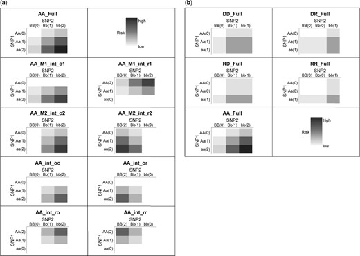
SNP–SNP interaction patterns of the AA9int and Five-Full approach. (a) Additive-additive 9 interaction-model approach (AA9int)¹. (b) Five full interaction model approach (Five-Full)¹. ¹Model label: D: dominant, R: recessive, A: additive (1st and 2nd letter represent inheritance mode for SNP1 and SNP2). Full: full interaction; M1_int: SNP1 main effect plus interaction; M2_int: SNP2 main effect plus interaction and ‘int’ only: model with an interaction only. o1, _r1: original coding (based on minor allele) for SNP1, and reverse coding for SNP1. _o2, _r2: original coding for SNP2, and reverse coding for SNP2. _oo, _or, _ro, _rr: based on original–original, original-reverse, reverse-original and reverse-reverse coding for SNP1–SNP2. The labels of two axes are ‘genotype (coding)’. A lowercase and capital letter denotes the minor and major allele, respectively. The darker the color, the higher the risk. These examples based on positive coefficients in SIPI models. If coding direction (‘o’/’r’) is not specified, the original coding is applied

2.4 Simulation

We conducted a simulation study to compare the power of Five-Full and AA9int with SIPI in detecting SNP–SNP interactions associated with disease risk (case/control), a binary outcome. For better comparison, the simulation settings and testing interaction models are the same as our previous SIPI study (Lin et al., 2017). We tested six interaction models with two different sample sizes (n = 1000 and 5000). The six testing models were simulated based on the designed SIPI models with positive model coefficients, which can be used to define high- and low-risk genotype sub-groups. The details of these six models are shown in Figures 2 and 3. Models 1–3 (RR_int_rr, DD_int_oo and RD_int_rr) are interaction-only models and the present outcome proportions for the high- and low-risk sub-groups are 0.3 and 0.2, respectively. The corresponding odds ratio (OR) is 1.7 for the high versus low risk groups. Model 4 (DD_M1_int_o1) is a model with both SNP1 main effect and an interaction where both SNPs have an original Dominant coding. The present outcome proportions were set up to be 0.2, 0.3 and 0.4 for low-, moderate- and high-risk sub-groups. The ORs are 1.7 and 2 for the moderate- and high-risk groups compared to the low-risk groups. Model 5 (AA_Full) is a full interaction model where both SNPs have an original additive coding. This model was based on β₀ = –2.5 and β₁= β₂= β₃= 0.6 in Equation (1). Model 6 (RD_int_oo) is an interaction-only model simulated based on the real data with an OR of 1.9. The two testing SNPs were generated independently based on the Hardy–Weinberg equilibrium, and their minor allele frequencies (MAF) are (0.5, 0.3), (0.5, 0.2) and (0.5, 0.05). We generated the binary outcome variable based on the present outcome proportion in each genotype combination of the two given SNPs using multi-nomial distribution. All analyses were based on 1000 simulation runs. Both power and Type I errors were compared. Statistical significance is based on the Bonferroni correction for multiple comparison justification.

Fig. 2.

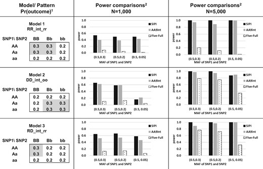
Power comparison of AA9int, Five-Full and SIPI for Models 1–3. ¹Model label: RD_int_rr (Interaction-only model with reverse-Rec SNP1 and reverse-Dom SNP2), DD_int_oo (Interaction-only model with original-Dom SNP1 and original-Dom SNP2) and RD_int_rr (Interaction-only model with reverse-Rec SNP1 and reverse-Dom SNP2). Values in the 3 x 3 table are present outcome proportions (such as disease prevalence). A lowercase and capital letter denotes the minor and major allele, respectively. ²SIPI (SNP Interaction Pattern Identifier), AA9int (Additive-additive nine interaction-model approach) and Five-Full (Five full interaction-model approach). MAF: minor allele frequency

Fig. 3.

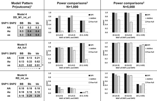
Power comparison of AA9int, Five-Full and SIPI for Models 4–6. ¹Model label: DD_M1_int_o₁ (Model with SNP1 main effect plus interaction with original-Dom SNP1 and Dom SNP2), AA_Full (Full interaction model with Add SNP1 and Add SNP2) and RD_int_oo (Interaction-only model with original-Rec SNP1 and original-Dom SNP2). Values in the 3 x 3 table are present outcome proportions (such as disease prevalence). A lowercase and capital letter denotes the minor and major allele, respectively. ²SIPI (SNP Interaction Pattern Identifier), AA9int (Additive-additive nine interaction-model approach) and Five-Full (Five full interaction-model approach). MAF: minor allele frequency

2.5 Application on prostate cancer aggressiveness

AA9int, the better approach compared to Five-Full based on the simulation results, was applied for this prostate cancer (PCa) application. We applied this AA9int approach to identify SNP–SNP interactions associated with PCa aggressiveness in the same PCa data used for our previous study (Lin et al., 2017). We evaluated the 148 SNPs in the six genes involved in the angiogenesis pathway (EGFR, MMP16, ROBO1, CSF1, FBLN5 and HSPG2), which were reported in a genetic interaction network associated with PCa aggressiveness (Lin et al., 2013). Aggressive PCa is defined as a Gleason score > 8, PSA >100, disease stage of ‘distant’ (stage IV) or death from PCa. There were 21 316 PCa cases of European ancestry from the 32 study sites in the Prostate Cancer Association Group to Investigate Cancer Associated Alterations in the Genome (PRACTICAL) consortium cohort. We randomly selected half of the subjects in the discovery set and the other half in the validation set in each study site. AA9int was applied in the discovery set (n = 10 664). In this discovery set, there were 1991 patients (18.7%) with aggressive PCa. In our previous study, there were 25 top SNP pairs associated with PCa aggressiveness with P-value < 0.001 in the discovery set using the SIPI approach. The coverage of selected SNP pairs using AA9int compared with SIPI was reported. For demonstrating the impact of various interaction patterns and approaches (Five-Full, AA9int and SIPI) on SNP–SNP interactions, we presented the P-values of the 45 interaction patterns of rs2075110 and rs7538029 in EGFR gene associated with PCa aggressiveness in the combined dataset. These SNP pairs have been shown to be associated with PCa aggressiveness in both discovery and validation sets (Lin et al., 2017).

2.6 Software

Our study results demonstrated that the AA9int approach performed better than Five-Full. Thus, the AA9int approach is to be used as the mini-version of SIPI to be applied alone or to serve as the screening tool prior to use SIPI (AA9int+ SIPI). The new function of ‘AA9int’ and ‘parAA9int’, the standard and parallel computing version of AA9int, are added in the SIPI R package. This software is freely available at https://linhuiyi.github.io/LinHY_Software/.

3 Results

3.1 Simulations

The power of AA9int is similar to that of SIPI, and both of them performed much better than Five-Full. In the majority of conditions, the rank of power for detecting a SNP–SNP interaction is SIPI≥ AA9int > Five-Full. AA9int is more powerful than Five-Full in the majority of the testing conditions (Figs 2 and 3). Using Model 1 with a sample size of 1000 and the MAF combination of (0.5, 0.05) for the two SNPs as an example, the power of AA9int and Five-Full is 0.43 and 0.02, respectively. Under the same setting in Model 1 with an increasing sample size to 5000, the power of AA9int increased to 0.99 but the power of Five-Full was still low (0.01). In Model 1, Five-Full also had low power in other testing conditions (0.04–0.21), including common variants and a large sample size. This demonstrates that the Five-Full approach failed to detect this interaction-only pattern.

Even when the true underlying model is AA-Full (Model 5), which is one testing pattern in both AA9int and Five-Full, AA9int is still more powerful than Five-Full, especially for a small sample size and SNPs with a low MAF. For Model 5 and MAF of two SNPs of (0.5 and 0.05), power of AA9int and Five-Full is 1.0 and 0.17, for a sample size of 1000 and power of both is close to 1 when the sample size increased to 5000.

The power of both Five-Full and AA9int to detect interactions of rare variants (with a low MAF) is lower than that of common SNPs, especially for studies with a small sample size. As shown in Figures 2 and 3, Five-Full had a larger penalty in detecting an interaction with rare variants than AA9int and SIPI. For Model 2 with a sample size of 5000, the power of SNPs with the MAF of (0.5, 0.2) and (0.5, 0.05) is 0.75 and 0.35 (reduce 0.4 power) for Five-Full, and the power for AA9int and SIPI only reduced to a power of 0.05 and 0.13 under the same conditions.

For some conditions (Models 2, 4, 5 with a small sample size of 1000), AA9int tends to be similar or more powerful than SIPI. For Model 2 with a MAF of (0.5, 0.05) and a sample size of 1000, power of AA9int is larger than one of SIPI (0.22 > 0.16). For Model 4 with a MAF of (0.5, 0.3) and a sample size of 1000, power of AA9int and SIPI is 0.84 and 0.73, respectively. For type I error comparison, these three methods were adjusted for multiple comparisons based on the Bonferroni corrections. As shown in Supplementary Figure S2, all type I errors were less than 0.05, which results from the conservative Bonferroni correction. The higher number of testing models, the lower the type I errors.

3.2 PCa example

We applied AA9int to test SNP–SNP interactions from a total of 148 SNPs (with 10 878 SNP pairs) associated with PCa aggressiveness in the discovery set of the PCa study. As we reported previously (Lin et al., 2017), there were 25 SNP pairs with a P < 0.001 selected using SIPI. Using AA9int, there are only two SNP pairs with the same criterion of a P-value < 0.001. When using AA9int with a cut-off P-value < 0.05 and <0.1, 1095 and 2557 SNP pairs were identified, respectively. Among the top 25 SNPs selected in SIPI, AA9int with a cut-off P-value < 0.05 and <0.1 can detect the 18 (72%) and 23 (92%) SNP pairs. This showed that AA9int with a liberal cut-off can be used as a good screening tool for SIPI.

As for computation time for analyzing all 10 878 pairs for a dataset with a sample size of 10 664 using the parallel computing version, AA9int spent only 21% computing time compared with SIPI (27 and 126 min, respectively) on a desktop computer with 3.0 GHz CPU and 8 cores. For the two-stage approach (AA9int+ SIPI) under the same conditions, it took 40 and 57 min for detecting SNP interactions for using a cut-off P-value < 0.05 and <0.1, respectively. In this example, AA9int with the cut-off P-value of 0.05 and 0.1 can detect 72–92% of the SIPI identified SNP pairs. Compared with SIPI, AA9int alone spent 21% computing time and the two-stage AA9int+ SIPI approach spent 32–45% computing time. For testing feasibility, we also evaluated performance of AA9int and SIPI (parallel computing version) for a dataset with a sample size of 10 350 and 100 000 SNP pairs. SIPI spent 23 h and 57 min and AA9int only took 4 h 51 min (20% time) to finish this task in a supercomputer (ratio of core used for parallel computing = 0.5, two 10-core 2.8 GHz E5-2680v2 Xeon processors and 64 GB memory).

To demonstrate the impact of both the interaction patterns and performance of AA9int and SIPI, the P-values of the 45 SIPI models for two EGFR SNPs (rs2075110 and rs7538029) associated with PCa aggressiveness in the combined dataset were presented in Table 3. With the conventional AA-Full approach, the P-value of this SNP pair associated with PCa aggressiveness is 0.138. Using the Five-Full, AA9int and SIPI approach, the P-values are 0.011, 0.002 and 2.6 x 10⁻⁵, respectively.

Table 3.

P-values of the SIPI 45 models for testing the interaction of two EGFR SNPs (rs2075110 and rs7538029) associated with PCa aggressiveness

Model Label	AA	DD	DR	RD	RR
Full	0.138	0.995	0.608	0.011(f)	0.107
M1_int_o1	0.053	0.005	0.043	0.526	0.620
M1_int_r1	1.7 x 10−4	0.085	0.523	3.5 x 10−5	0.009
M2_int_o2	0.581	0.794	0.553	0.247	0.195
M2_int_r2	0.131	0.753	0.767	0.008	0.098
int_oo	0.028	0.005	0.040	0.829	0.802
int_or	0.904	0.033	0.702	0.155	0.158
int_ro	0.002(a)	0.227	0.581	0.001	0.014
int_rr	0.003	0.146	0.581	2.6 x 10−5(s)	0.023

Note: A: additive; D: dominant; R: recessive mode. Full-int: full interaction model with two main effects plus an interaction; Main1+int: main effect of variable 1 plus an interaction; Main2+int: main effect of variable 2 plus an interaction and (4) Int-only: an interaction only. Coding direction: ‘o1’ (original for SNP1), ‘o2’ (original for SNP2), r1’ (reverse for SNP1), ‘r2’ (reverse for SNP2), ‘oo’ (original–original for SNP1-SNP2), ‘or’ (original-reverse), ‘ro’ (reverse-original), and ‘rr’ (reverse-reverse).The selections of SIPI, AA9int and Five-Full were in bold with a label of (s), (a) and (f), respectively.

4 Discussion

Based on our simulation results, it is clearly shown that non-hierarchical models play a more important role in SNP interaction detection than inheritance modes. AA9int has similar statistical power compared to SIPI and is superior to Five-Full in detecting SNP–SNP interactions associated with a binary outcome. Five-Full acted poorly for SNP pairs with a small sample size, rare variants and non-hierarchical true model structure. Using Model 1 as an example, this model has the RR_int_rr pattern, which is an interaction-only model with SNP1 with reverse-recessive coding and SNP2 with reverse-recessive coding. Model 1 has the interaction pattern with two risk genotype sub-groups: AA/Aa + BB/Bb versus other genotypes with at least aa or bb. Among the Five-Full, the closest model is RR_Full, which tests four distinct risk sub-groups [(AA/Aa + BB/Bb), (AA/Aa ± bb), (aa + BB/Bb), (aa+ bb)]. The last three sub-groups had a small sample size and a low risk, so this made it more difficult to show distinct risk of these three sub-groups by random. This is the reason why Five-Full had little power detecting the Model 1 interaction pattern.

For the full interaction models for two SNPs, three degrees of freedom are needed in modeling; therefore four unique sub-groups are compared for the binary modes (Dom and Rec, Fig. 1b). It is nature to have unstable interaction patterns because of nine genotype combinations for testing pairwise SNP interactions. Even though the true underlying interaction pattern is the full interaction pattern, the interaction pattern in the testing data may reduce to a lower number of distinct sub-groups (such as two or three) than the truth for a SNP pair with a small sample size and/or rare variants. The non-hierarchal interaction structures provide a useful feature to solve this unstable pattern issue. Using Model 5 (AA_Full) as an example, the true underlying model is the additive-additive full interaction model. With a small sample size and a SNP with a rare variant [n = 1000 and MAF = (0.5, 0.05)], the Five-Full approach had low statistical power compared with AA9int (power = 0.17 versus 1, respectively). As shown in Supplementary Figure S1a–1c, the non-hierarchal interaction structure allows the cells (individual genotype combinations) with a similar outcome prevalence or a small sample size to be combined. This explains why AA9int, which considers non-hierarchical interaction models, performs much better than Five-Full. Compared to the binary modes (dominant and recessive), the additive mode shows the risk pattern in an ordinal way (Supplementary Fig. S1a–c). Thus, there are some similarities of risk patterns between additive modes and the other two binary modes. This explains why the AA9int approach can be treated as an excellent screening method for SIPI.

In addition, we are interested in comparing AA9int and Five-Full with other two common approaches: MDR and Additive-Additive full interaction models (AA-Full). With the same simulation settings, we can compare the results of AA9int with the MDR and AA-Full results, which were reported previously. Five-Full has similar statistical power compared with conventional AA-Full (Lin et al., 2017). That is, SIPI≥ AA9int ≥ Five-Full ≈ AA-Full for detecting SNP–SNP interactions. AA9int has similar power to SIPI and MDR. Using Model 2 with a sample size of 1000 and the MAF combination of (0.5, 0.2) for the two SNPs as an example, the power of AA9int, SIPI and MDR is 0.59, 0.58 and 0.59 and power of Five-Full and AA-Full is 0.13 and 0.19, respectively. Five-Full includes four additional modes (Dom–Dom, Dom-Rec, Rec-Dom and Rec–Rec), but did not improve too much in terms of power of SNP interaction detection compared with AA-Full. Based on our previous studies (Lin et al., 2008, 2013), the majority of the selected SNP pairs are interaction-only patterns, especially for studies with a small sample size. This supports the importance of considering non-hierarchical models in SNP interaction detection.

For application, researchers can use pathway analyses to select candidate SNPs for interaction analyses. The SNP interaction pairs, identified using AA9int or AA9int+SIPI, can be applied as components to build prediction models or genetic risk scores. The genetic models or scores with SNP interaction pairs tend to have better performance than the ones with only main effects. The strengths of the AA9int approach are (i) a powerful and computationally feasible way to detect SNP–SNP interactions, (ii) easy interpretation using interaction patterns and (iii) can be used for building predicted models or scores. The weakness of AA9int or AA9int+ SIPI is potential high false positive findings. As we expected, a powerful approach increases its true positive rate but also increases its false positive rate. Thus, external validation using an independent set and further laboratory experiments will be needed to confirm true biological interactions.

Although AA9int is not as powerful as SIPI, AA9int is more computational feasible for testing SNP–SNP interactions. Based on our PCa project, AA9int can successfully identified 72–92% candidate SNP pairs and only use ∼20% computation time compared to SIPI. Different from other software, both AA9int and SIPI can allow the users to input the candidate ‘pairs’ or candidate SNPs. This feature can significantly reduce the amount of computation time for limiting analyses on candidate SNP ‘pairs’ instead of all possible pairs of candidate SNPs. This study also clearly demonstrates that interaction patterns have a dramatic impact on SNP–SNP interaction detection. Using statistical methods without considering non-hierarchical interaction model structures, studies will suffer false negative findings and lose the chance to detect true interaction signals. In summary, AA9int is not meant to replace the original SIPI but provides a computationally efficient and still effective tool. For large-scale genetic studies, the two-stage method (AA9int + SIPI) is a feasible and powerful approach for detecting SNP–SNP interactions.

Acknowledgements

The authors gratefully acknowledge use of the computing facilities at School of Public Health, Louisiana State University Health Sciences Center. Portions of this research were conducted with high performance computational resources provided by the Louisiana Optical Network Infrastructure (http://www.loni.org).

Funding

This study was supported by the National Cancer Institute (R21CA202417, PI: Lin, HY).

Conflict of Interest: none declared.