BMC3C: binning metagenomic contigs using codon usage, sequence composition and read coverage

Abstract

Motivation

Metagenomics investigates the DNA sequences directly recovered from environmental samples. It often starts with reads assembly, which leads to contigs rather than more complete genomes. Therefore, contig binning methods are subsequently used to bin contigs into genome bins. While some clustering-based binning methods have been developed, they generally suffer from problems related to stability and robustness.

Results

We introduce BMC3C, an ensemble clustering-based method, to accurately and robustly bin contigs by making use of DNA sequence Composition, Coverage across multiple samples and Codon usage. BMC3C begins by searching the proper number of clusters and repeatedly applying the k-means clustering with different initializations to cluster contigs. Next, a weight graph with each node representing a contig is derived from these clusters. If two contigs are frequently grouped into the same cluster, the weight between them is high, and otherwise low. BMC3C finally employs a graph partitioning technique to partition the weight graph into subgraphs, each corresponding to a genome bin. We conduct experiments on both simulated and real-world datasets to evaluate BMC3C, and compare it with the state-of-the-art binning tools. We show that BMC3C has an improved performance compared to these tools. To our knowledge, this is the first time that the codon usage features and ensemble clustering are used in metagenomic contig binning.

Availability and implementation

The codes of BMC3C are available at http://mlda.swu.edu.cn/codes.php?name=BMC3C.

Supplementary information

Supplementary data are available at Bioinformatics online.

1 Introduction

Metagenomics has brought insights into the diversity, metabolism and ecology of the uncultivated microbial majority (Riesenfeld et al., 2004). It has been extensively used to study microbial communities in both natural (Tyson et al., 2004; Venter et al., 2004) and man-made environments (García et al., 2006). The key step of metagenomic data analysis is to assemble short metagenomic reads into long genomic fragments or contigs. However, assembly often fails to produce full-length genomes or significant parts of the genome (Alneberg et al., 2014). Thus, metagenomic contigs binning methods have been developed to classify metagenomic contigs into genome bins.

The available metagenomic contigs binning methods fall into three categories (Sangwan et al., 2016): (i) nucleotide composition (NC-) based, (ii) coverage-based and (iii) nucleotide composition and coverage (NCC-) based. NC-based methods make use of oligonucleotide frequency variations among microbial lineages. These methods are often supervised, and they assign contigs to taxonomic groups by comparing metagenomic sequences to reference databases. Most of them employ conventional machine learning approaches, such as interpolated Markov models (IMMs) (Brady and Salzberg, 2009), k-nearest neighbors (kNN) classifier (Diaz et al., 2009), naive Bayesian classifier (NBC) (Rosen et al., 2011) and support vector machine (SVM) (McHardy et al., 2007) among other classifiers. For instance, TACOA (Diaz et al., 2009) extends traditional kNN by introducing a Gaussian kernel. PhyloPythia (McHardy et al., 2007) trains SVM using the oligonucleotide composition of genomic fragments with varying lengths and applies the all-versus-all technique to solve the multi-species binning problem. Phymm (Brady and Salzberg, 2009) uses IMMs to characterize variable-length k-mers of a phylogenetic group and then handles the general phylogenetic classification problem. PhymmBL (Brady and Salzberg, 2009) is a successor of Phymm, which combines the results of BLAST with scores produced by IMMs to improve the accuracy. On the other hand, coverage-based methods rely on the differential abundance of contigs across multiple samples (Sangwan et al., 2016). These methods were successfully applied to solve real-world problems. For instance, Sharon et al. (Sharon et al., 2013) reconstructed six complete and two nearly complete bacterial genomes using emergent self-organizing maps to cluster scaffolds. Nielsen et al. (2014) developed a coverage-based method called Canopy to reconstruct microbial phage and plasmid genomes using co-abundance patterns across multiple samples. Canopy clusters contigs by randomly picking a seed gene from the community gene pool and clusters genes with similar co-abundance profiles using strict pairwise correlation cutoff.

While NC-based and coverage-based methods have led to a variable success in solving real-world problems (Nielsen et al., 2014; Sharon et al., 2013), NCC-based methods combine the characteristic of nucleotide composition and coverage, and thus often outperform the former methods (Sangwan et al., 2016). NCC-based methods generally employ clustering approaches to bin contigs instead of short reads, since binning contigs is more reliable than binning short reads (Nolla-Ardèvol et al., 2015). In addition, clustering approaches are unsupervised, which do not need reference databases or taxonomic information. For instance, CONCOCT (Alneberg et al., 2014) uses Gaussian mixture model to cluster metagenomic contigs and applies modified Bayesian model selection to automatically determine the number of clusters. MetaBAT (Kang et al., 2015) uses integrated distance of pairwise contigs based on tetranucleotide frequency and coverage patterns across samples to group contigs. It modifies k-medoid (Kaufman and Rousseeuw, 1987) clustering without a need to preset the number of clusters. MaxBin (Wu et al., 2014, 2016) empirically estimates Gaussian distributions of intra-/inter-genome distances and uses an expectation-maximization algorithm to bin contigs. COCACOLA (Lu et al., 2016) uses L1-norm distance, rather than Euclidean distance, to measure the similarity of pairwise contigs and applies Nonnegative Matrix Factorization (NMF) (Lee and Seung, 1999) to cluster contigs.

Despite the apparent advantage by making use of both nucleotide composition and sequence coverage, most NCC-based methods use a single clustering method. The problem of single clustering is that it cannot capture the cluster shapes and sizes for complex datasets like metagenomic contigs. We therefore develop BMC3C, an ensemble clustering method allows for exploring and capturing the complex structure of the metagenomic datasets by repeatedly performing clusterings on the datasets with different initializations or algorithms. By fusing the knowledge discovered by each base clustering, the ensemble method yields more accurate results that are less sensitive to the input parameters of base clustering methods (Strehl and Ghosh, 2002). Although ensemble clustering has been studied by the machine learning and data mining community for several decades, it has not been well explored for contigs binning. Moreover, five new independent features fully describing codon usage are introduced to BMC3C. In fact, the codon usage features have not been used in any other contig binning methods. Experimental results on simulated and real datasets demonstrate that BMC3C performs significantly better than state-of-the-art binning tools, including COCACOLA, CONCOCT, MetaBAT and MaxBin2.0, and also runs efficiently.

2 Materials and methods

2.1 Feature representation for metagenomic contigs

2.1.1 Composition and coverage

Composition considers the frequency variation of oligonucleotides among contigs, and Coverage is the representativeness of contigs across multiple samples (Sangwan et al., 2016). BMC3C uses a common practice like in (Alneberg et al., 2014; Lu et al., 2016) to represent composition and coverage. Suppose H is an n × w matrix, n is the number of contigs, and w is the number of distinct words. Using tetranucleotide (4-mer) frequency to represent the composition of contigs, there are 136 distinct words out of 4⁴ = 256 words in total after palindromic words (e.g. ATTA) are excluded. Let ${\mathbf{H}}_{i,j}$ be the j-th 4-mer of the i-th contig, to avoid zero entries which will affect the follow-up clustering, we simply add a pseudo-count to each 4-mer as ${\mathbf{H}}_{i,j}={\mathbf{H}}_{i,j}+1$⁠.

To reduce the length heterogeneity among contigs, we normalize the composition as follows:

$${\tilde{\mathbf{H}}}_{i,j}=\frac{{\mathbf{H}}_{i,j}}{{\sum }_{h=1}^w{\mathbf{H}}_{i,h}}$$

(1)

For Coverage, let R be an n × s matrix, where s is the number of metagenomic samples. To remove zero entries, let ${\mathbf{R}}_{i,j}={\mathbf{R}}_{i,j}+100/l{c}_i$⁠, lc_i is the length of the i-th contig. We also normalize R as follows:

$${\tilde{\mathbf{R}}}_{i,j}=\left(\frac{{\mathbf{R}}_{i,j}}{{\sum }_{i=1}^n{\mathbf{R}}_{i,j}}\right)/\left(\sum _{h=1}^s\frac{{\mathbf{R}}_{i,h}}{{\sum }_{i=1}^n{\mathbf{R}}_{i,j}}\right)$$

(2)

The denominator (⁠${\mathbf{R}}_{i,h}/{\sum }_{i=1}^n{\mathbf{R}}_{i,j}$⁠) is the column-wise normalization, which mitigates the heterogeneity of size (number of reads) among samples. The whole equation is row-wise normalization, which mitigates the heterogeneity of length among contigs.

2.1.2 Codon usage

There are 61 codons encoding 20 amino acids, and thus multiple codons may encode the same amino acid (i.e. codon degeneracy). Codon usage bias means synonymous codons are used unequally in protein-coding DNA among taxonomic groups. We use five independent statistics to measure codon usage of a protein-coding gene, and these statistics are derived from (Hughes and Langley, 2007). For a given protein-coding gene, TC2 is the number of 2-fold degenerate sites using T or C, and C2 is the number of C at these sites. Likewise, AG2 is the number of 2-fold degenerate sites using A or G, and G2 is the number of G at these sites. N4 represents the total number of 4-fold degenerate sites, while C4, G4 and A4 are the number of C, G and A at these sites, respectively. The five statistics are given as follows:

$$\begin{array}{c}PC2=\frac{C2}{TC2};\hspace{1em}PG2=\frac{G2}{AG2};\hspace{1em}PC4=\frac{C4}{N4}\hfill \\ PG4=\frac{G4}{N4};\hspace{1em}PA4=\frac{A4}{N4}\hfill \end{array}$$

(3)

where PC2 is the percentage of C in 2-fold degenerate sites using T or C; PG2 is the percentage of G in 2-fold degenerate sites using A or G; PC4, PG4 and PA4 represent the percentage of C, G and A at 4-fold degenerate sites, respectively.

We further modify these five statistics to represent all protein-coding DNA in a contig, instead of a gene. Suppose $n_g^i$ is the number of genes in the i-th contig, ${\mathbf{G}}_g^i=[PC{2}_g,PG{2}_g,\hspace{0.17em}PC{4}_g,PG{4}_g,PA{4}_g]$⁠, which represents the codon usage of the g-th gene in the i-th contig. The codon measurement for the i-th contig is defined as follows:

$${\mathbf{y}}_i=\frac{{\sum }_{g=1}^{n_g^i}{l}_g{\mathbf{G}}_g^i}{{\sum }_{g=1}^{n_g^i}{l}_g}$$

(4)

where l_g is the length of the g-th gene and the denominator is the total length of all genes in the i-th contig. The codon statistics matrix $\mathbf{Y}\in {ℝ}^{n\times 5}$ is $\mathbf{Y}=\left[{\mathbf{y}}_1;{\mathbf{y}}_2;\cdots ;{\mathbf{y}}_n\right]$⁠. We further normalize Y as ${\tilde{\mathbf{Y}}}_{i,c}={\mathbf{Y}}_{i,c}/{\sum }_{h=1}^n{\mathbf{Y}}_{h,c}$⁠.

To this end, we concatenate the data matrices describing Composition, Coverage and Codon usage into a numeric feature matrix as $\mathbf{X}=[\tilde{\mathbf{H}},\tilde{\mathbf{R}},\tilde{\mathbf{Y}}],\hspace{0.17em}\mathbf{X}\in {ℝ}^{n\times d}$⁠, where d = w + s + 5 is the total number of features. X will be used as the feature input of BMC3C for binning contigs.

2.2 Procedures of BMC3C

Unlike existing binning methods that merely use single clustering, BMC3C fuses the clustering results obtained by repeating k-means on the metagenomic datasets with different initializations. The whole procedure includes four phases, which are described in Figure 1. The following subsections elaborate on these phases.

Fig. 1.

The procedure of BMC3C. First, BMC3C searches the number of clusters. Second, BMC3C repeatedly applies k-means with different initializations to cluster contigs and produce multiple base clusterings. Next, results of these clusterings are used to build a weight graph with each node representing a contig and each edge reflecting the frequency of two connected nodes grouped into the same genome bins. Finally, a graph partitioning technique [Ncut (Shi and Malik, 2000)] is applied to partition the graph into some subgraphs, each corresponding to a genome bin

2.2.1 Search the number of clusters

We use a strategy modified from (Lu et al., 2016) to automatically determine the number of clusters. BMC3C initially sets k⁰ (not the final number of clusters) as the potential number of clusters. Next, it uses the separable conductance as the measure to search the underlying relationship between contigs. Let sep(k₁, k₂) be the separable conductance between the k₁-th cluster and the k₂-th cluster, sep(k₁, k₂) counts the contigs in the k₁-th cluster that are also included in the spherical scope of the k₂-th cluster. Here, spherical scope is defined as the third quartile among the intra-cluster distances. If sep(k₁, k₂) is large, the two clusters are highly relevant and not separable, and thus are merged into one cluster. On the contrary, if sep(k₁, k₂) is small, the two clusters have low relevance and are separable. BMC3C uses this criterion to iteratively merge clusters until the total number of clusters is smaller than a preset threshold, which indicates the structure of clusters tends to be stable. Next, BMC3C counts the number of remaining clusters and denotes it as $k^{*}$⁠, which is the number of potential clusters for ensemble clustering. The search procedure is described as follows:

• Perform k-means to get k⁰ clusters.

• Calculate the sep(k₁, k₂) for each pair of clusters. If sep(k₁, k₂) of two clusters exceeds a threshold, merge these two clusters. In the present study, the threshold is set as 1.

• After merging clusters, count the merged clusters and denote it as k_m.

• If $k_m<=0.85*k^0$⁠, then $k^0=k_m$ and goto step (ii); otherwise, set the number of clusters as $k^{*}=k_m$⁠.

2.2.2 k-means

This subsection elaborates on the k-means algorithm (MacQueen, 1967), which serves as the base clustering in BMC3C. Suppose $\mathbf{X}=[{\mathbf{x}}_1;{\mathbf{x}}_2;{\mathbf{x}}_3;\cdots ;{\mathbf{x}}_n]$ is a dataset with n contigs, ${\mathbf{x}}_n\in {ℝ}^d$ is a d-dimensional vector that represents feature information of a contig, and k(< n) is the specified number of clusters for k-means. Note, k for the base k-means clustering is not the final number of clusters (⁠$k^{*}$⁠) for BMC3C, and also not the k⁰ used to estimate $k^{*}$⁠. It is an adjustable parameter and set as $k=10\times k^{*}$ throughout this study. The reason for this setup is that a large k can better reflect the underlying local structure of a dataset than a small k. In an extreme case, each contig forms a cluster by itself if k = n, and the relationships among contigs cannot be calculated. For this reason, we ensure k < n. k-means aims to group n contigs into k clusters by minimizing an objective function described as follows:

$$argmin\sum _{h=1}^k\sum _{{\mathbf{x}}_i\in {\mathcal{C}}_h}{\Vert {\mathbf{x}}_i-{\mathbf{u}}_h\Vert }^2$$

(5)

where ${\mathcal{C}}_h$ is the h-th cluster, ${\mathbf{x}}_i$ is the i-th contig and ${\mathbf{u}}_h$ is the geometric centroid of the contigs in ${\mathcal{C}}_h$⁠.

After performing k-means to group X into k clusters, an n × 1 label vector is generated by k-means. We expand this label vector into an n × k label indicator matrix M. Entry ${\mathbf{M}}_{i,h}$ indicates the membership of a contig, with ${\mathbf{M}}_{i,h}=1$ specifying the i-th contig in the h-th cluster, and ${\mathbf{M}}_{i,h}=0$ otherwise. ${\sum }_{h=1}^k{\mathbf{M}}_{i,h}=1$ ensures the i-th contig exclusively belonging to one particular cluster.

However, k-means suffers from several issues. One issue is that a single k-means may not capture the underlying structure of complex datasets, such as metagenomics contigs. To illustrate this issue, we project two simulated datasets (Species and Strain) and a real-world dataset (Sharon) into 2-dimensional subspace via principal component analysis (PCA) (Jolliffe, 1986). These datasets are also used in the subsequent experimental study to compare the performance of BMC3C and other available tools. We show that the distribution of contigs of different species (or strains) are heavily overlapped (Fig. 2). As such, it is difficult for a single k-means to reveal the underlying structure of these metagenomic datasets. Another issue is that k-means randomly selects k initial centroids of the clusters, but the choice of the centroids may have a major impact on the final clustering results. In fact, these issues are also associated with other binning methods that apply single clustering in one round (Lu et al., 2016; Sangwan et al., 2016).

Fig. 2.

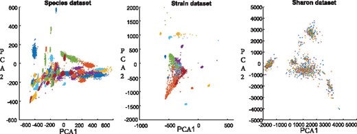
Two-dimensional visualization of a simulated Species dataset, a simulated Strain dataset and a real-world Sharon dataset. Each color corresponds to a species or a strain. The distributions of contigs in all datasets are very irregular. For Species and Strain datasets, only few clusters are separated while most clusters are overlapped. For Sharon dataset, almost all clusters are overlapped. PCA1 and PCA2 are the first two dimensions of the datasets after using principal component analysis (PCA)

2.2.3 Ensemble k-means

As ensemble clustering can be viewed as an evidence-accumulating or knowledge-reusing process (Fred and Jain, 2005; Strehl and Ghosh, 2002), it generally leads to more stable and effective results than its base clustering and thus may alleviate the issues intrinsic to the base clustering. Here, the ensemble method BMC3C performs k-means m times with a fixed k. To integrate the results from independent k-means, a co-association matrix $\mathbf{W}\in {ℝ}^{n\times n}$ is defined as follows:

$$\mathbf{W}=\left(\sum _{t=1}^m{\mathbf{S}}_t\right)/m$$

(6)

where ${\mathbf{S}}_t$ is the t-th clustering observation matrix and is computed as follows:

$${\mathbf{S}}_t={\mathbf{M}}_t{\mathbf{M}}_t^T$$

(7)

where ${\mathbf{M}}_t\in {ℝ}^{n\times k}$ is the cluster indicator matrix of the t-th base clustering. Here, ${\mathbf{S}}_t(i,j)=1$ if ${\mathbf{x}}_i$ and ${\mathbf{x}}_j$ share the membership of the same cluster by the t-th k-means clustering, and ${\mathbf{S}}_t(i,j)=0$ otherwise. From this perspective, W can be viewed as the weighted adjacency matrix of a graph, it accumulates the co-association evidence between pairwise contigs carried by m base clustering. Thus, W represents the algebraic connectivity of n contigs. If two contigs are frequently grouped into the same clusters, they likely share the membership of the same genome bins.

Since the co-association relationship between n contigs is encoded by a graph, the graph partitioning technique normalized cut (NCut) (Shi and Malik, 2000; Yu and Shi, 2003) is employed to partition it into subgraphs, each of which corresponds to a cluster of contigs or a genome bin. Given a graph $G=(\mathcal{V},\mathbf{W})$⁠, where $\mathcal{V}$ is the set of contigs, and W is the weighted adjacency matrix and obtained from Eq. (6). Let $\mathcal{A},\mathcal{B}\subseteq \mathcal{V}$ be two subgraphs, and $links(\mathcal{A},\mathcal{B})$ be the total weight edges between $\mathcal{A}$ and $\mathcal{B}$⁠:

$$links(\mathcal{A},\mathcal{B})=\sum _{i\in \mathcal{A},j\in \mathcal{B}}\mathbf{W}(i,j)$$

(8)

Then the normalized link ratio of $\mathcal{A}$ and $\mathcal{B}$ is:

$$linkratio(\mathcal{A},\mathcal{B})=\frac{links(\mathcal{A},\mathcal{B})}{links(\mathcal{A},\mathcal{V})}$$

(9)

In particular, $linkratio(\mathcal{A},\mathcal{A})$ measures the number of links staying within $\mathcal{A}$⁠, and $linkratio(\mathcal{A},\mathcal{V}\setminus \mathcal{A})$ measures the number of links escaping from $\mathcal{A}$⁠. A desirable clustering features tight connections within a subgraph and loose connections between subgraphs (Yu and Shi, 2003). These two goals are extendable for the ‘multi-class’ normalized cut problem, which simultaneously maximizes the links in a cluster and minimizes the links that escape a cluster as follows:

$$\underset{{\mathcal{V}}_h}{\mathrm{argmin}}\frac{1}{k^{*}}\sum _{h=1}^{k^{*}}linkratio({\mathcal{V}}_h,\mathcal{V}\setminus {\mathcal{V}}_h)$$

(10)

where $k^{*}$ is the sought number of clusters in the previous subsection, and ${\mathcal{V}}_h$ includes the contigs of the h-th cluster. From Eq. (10), we can find that NCut not only maximizes links of internal subgraph, but also minimizes links of external subgraphs. This is consistent with the idea of clustering by viewing each subgraph as a cluster. Therefore, BMC3C uses the graph partitioning technique to further cluster contigs based on the structure of G. The normalized cut criterion can be simplified as the following trace maximization problem (Yu and Shi, 2003):

$$\underset{\mathbf{U}}{\mathrm{argmax}}\hspace{0.17em}tr\left({\left(\mathbf{U}{({\mathbf{U}}^T\Lambda U)}^{-\frac{1}{2}}\right)}^T\mathbf{W}\right(\mathbf{U}{({\mathbf{U}}^T\Lambda U)}^{-\frac{1}{2}}\left)\right)$$

(11)

where $\mathbf{\Lambda }\in {ℝ}^{\mathit{n}\times \mathit{n}}$ is a diagonal matrix, whose diagonal entries are spanned by the row sum of W, and $\mathbf{U}=[{\mathbf{U}}_1,{\mathbf{U}}_2,\dots ,{\mathbf{U}}_{k^{*}}]\in {ℝ}^{n\times k^{*}}$⁠. In fact, ${\mathbf{U}}_h$ is a binary indicator vector for vertices in ${\mathcal{V}}_h$⁠. If vertex i is divided into ${\mathcal{V}}_h,\hspace{0.17em}{\mathbf{U}}_h\left(i\right)=1$⁠, otherwise ${\mathbf{U}}_h\left(i\right)=0$⁠. However, finding a discrete solution in Eq. (11) is an NP-hard problem. Here, we use an approximate nearby discrete solution. Let $\mathbf{P}=\mathbf{U}{({\mathbf{U}}^T\Lambda U)}^{-\frac{1}{2}}$⁠, a natural constraint on P is ${\mathbf{P}}^T\Lambda P={\mathbf{I}}_{k^{*}}$⁠, where ${\mathbf{I}}_{k^{*}}$ denotes the $k^{*}\times k^{*}$ identity matrix. Let ${\mathbf{P}}^{*}={\mathbf{\Lambda }}^{\frac{1}{2}}\mathbf{P}$ and relax U as a numeric matrix, the trace minimization problem can be obtained as follows:

$$\underset{{\mathbf{P}}^{*}}{\mathrm{argmin}}\hspace{0.17em}tr\left({\mathbf{P}}^{*T}{\mathbf{\Lambda }}^{-\frac{1}{2}}\mathbf{W}{\mathbf{\Lambda }}^{-\frac{1}{2}}{\mathbf{P}}^{*}\right)$$

(12)

where the constraints on ${\mathbf{P}}^{*}$ are relaxed such that ${\mathbf{P}}^{*T}{\mathbf{P}}^{*}={\mathbf{I}}_{k^{*}}$⁠. A well-known solution to this problem can be achieved by setting ${\mathbf{P}}^{*}$ as the top $k^{*}$ eigenvectors of the matrix ${\mathbf{\Lambda }}^{-\frac{1}{2}}\mathbf{W}{\mathbf{\Lambda }}^{-\frac{1}{2}}$⁠. Discrete partition of U will be computed by these eigenvectors. More details of the optimization of Eq. (12) can be found in (Yu and Shi, 2003).

3 Results and discussion

3.1 Datasets

We use two simulated metagenomic datasets publically available from (Alneberg et al., 2014) and five real-world metagenomic datasets for experiments. These simulated datasets are at Species and Strain levels, respectively. The Species dataset simulates 101 different species across 96 samples originated from Human Microbiome Project (Human Microbiome Project Consortium, 2012). The Strain dataset simulates 20 strains from 64 samples also originated from Human Microbiome Project. The five real-world microbiome datasets are Sharon dataset with 11 fecal samples (Sharon et al., 2013), HMP dataset with 10 human samples (Human Microbiome Project Consortium, 2012), Human gut dataset with 264 samples (Qin et al., 2010), Amazon dataset with three Amazon river plume samples (Satinsky et al., 2014) and Chronic Obstructive Pulmonary Disease (COPD) dataset with eight sputum samples (Cameron, 2016). Further information of these datasets is provided in the Supplementary Material.

As contigs rather than the reads are used for binning, reads are first assembled into contigs using SPAdes (Bankevich et al., 2012), followed by open reading frame (ORF) calling using Prodigal (Hyatt et al., 2010). Only contigs with at least 1000 bp and one predicted ORF are retained for binning. This procedure led to 37 585, 9401, 2886, 2654, 46 434, 157 960 and 192 673 contigs in the Species, Strain, Sharon, COPD, Amazon, HMP and Human gut datasets, respectively. It is common that metagenomic contigs contain incomplete ORFs. To reduce the impact of incomplete ORFs, BMC3C keeps ORFs with at least 33 codons (99 bp) for codon usage analyses.

For the simulated datasets, contigs are automatically labeled with known taxonomy. If a contig is chimeric (i.e. the co-assembly of reads from different taxonomic groups), it is labeled with the taxonomic group that dominates the reads comprising this contig. For the real-world dataset, we follow the procedure in evaluating other binning tools (Alneberg et al., 2014; Lu et al., 2016), in which contigs are labeled using TAXAassign v0.4 (https://github.com/umerijaz/taxaassign), which uses BLAST to search matches in the NCBI nucleotide database with a given identity and query coverage. For the Sharon, HMP and Human gut datasets, this procedure led to unambiguously labeling of 2069, 18 081 and 15 011 contigs, respectively, each with at least 1000 bp and one predicted ORF. For the Amazon and the COPD datasets, however, only 202 and 220 contigs were labeled, respectively, likely because of less available representative reference genomes in the database.

We use three representative evaluation metrics, precision, recall and Adjusted Rand Index (ARI), to evaluate the clustering results. The formal definitions of these metrics are described in the Supplementary Material.

3.2 Results on simulation datasets

The performance of BMC3C is compared to that of four representative NCC-based methods, COCACOLA (Lu et al., 2016), CONCOCT (Alneberg et al., 2014), MetaBAT (Kang et al., 2015) and MaxBin2.0 (Wu et al., 2016). All these methods can automatically search the final number of clusters $k^{*}$⁠, but BMC3C, COCACOA and CONCOCT need to initialize the maximum number of clusters, which is uniformly set as $k^0=n*0.006$⁠, where n is the number of contigs. In fact, $n*0.006$ is an upper bound of k⁰, but users can assign other values to k⁰. In addition, BMC3C repeats k-means 50 times each with a distinct initialization of centroids and subsequently takes these 50 base clusterings for ensemble analysis. Other parameters of these comparing methods are adopted with the default values that are provided in the original codes. Figure 3 reports the performance of the five methods with respect to the three metrics ARI, precision and recall using the Species and Strain datasets. In general, all methods except COCACOLA have a better performance using the Species dataset than the Strain dataset.

Fig. 3.

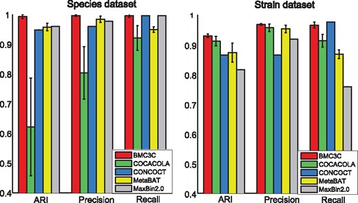
Results of BMC3C and other four binning methods (COCACOLA, CONCOCT, MetaBAT and MaxBin2.0) on two simulated datasets are shown with regards to ARI, Precision and Recall. Left: Species dataset; Right: Strain dataset

COCACOLA is very unstable on the Species dataset, it uses NMF and needs to initialize two non-negative low-rank matrices, but different initializations often have an impact on the final clustering results. In practice, COCACOLA uses k-means for initialization, and thus its performance depends on k-means, which is known to have a decreasing performance as the datasets become increasingly large and complex. Consistent with this, the Species dataset (37 585 contigs from 101 species) is larger and more complex than the Strain dataset (9401 contigs from 20 strains), which may explain why COCACOLA on the Species dataset is less stable than that on the Strain dataset. While MetaBAT has a precision similar to BMC3C, it has reduced ARI and recall compared to the latter. This may be related to the fact that MetaBAT uses a modified k-medoid clustering, which initializes the centroids in a random way as k-means works. BMC3C has the best performance among all methods in terms of the three metrics. It also has a reduced variance compared to all other methods except CONCOCT and MaxBin2.0. We are not able to determine the variance of the CONCOCT and MaxBin2.0 results, because these methods use the same initialization at each clustering. One possible reason leading to the success of BMC3C is that this ensemble clustering fuses the results from multiple base clusterings generated by separate k-means, allowing for more accurately capturing the underlying structure of the complex datasets. Another possible reason is that BMC3C uses five independent statistics of codon usage as new features to represent contigs, which are not used in all other binning methods.

3.3 The effect of codon usage

To investigate the effect of codon usage, we compare the performance of BMC3C with/without the use of codon usage features and use CONCOCT (Alneberg et al., 2014) as a reference. We show that incorporation of the codon usage features improves the performance of BMC3C on both Species and Strain datasets (Fig. 4). The differential use of synonymous codons (or codon usage bias) is the result of a balance between selection for translational efficiency/accuracy and mutational bias (Bulmer, 1991). It is a phylogenetically independent feature that can be calculated without a need for reference genomes, and thus contributes to contig binning at a finer phylogenetic resolution. Likewise, we observe an improved performance of CONCOCT with the inclusion of the codon usage features, suggesting that codon usage can also work with other binning methods.

Fig. 4.

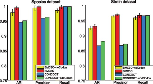
Results of BMC3C and CONCOCT each with/without the use of codon usage features on two simulated datasets are shown with regards to ARI, Precision and Recall. Left: Species dataset; Right: Strain dataset

We also investigated the effect of ensemble k-means and tuning the weights of three types of features (Coverage, Composition and Codon usage), and the detailed results of these experiments are presented in the Supplementary Material. Overall, the ensemble clustering significantly improves the robustness and accuracy of binning compared to every single clustering (Supplementary Fig. S2), and the weight experiment shows that the coverage and the composition features are more informative than the codon usage features. However, including the codon usage features further improves the performance of BMC3C (Supplementary Fig. S4). We also observe that different datasets have different optimal weights. For simplicity, BMC3C equally weights the three types of features, and its performance can be further improved by tuning the weights.

3.4 Results on real-world datasets

We further compare BMC3C with four related binning methods on the five real-world datasets. For the Sharon dataset, the maximum number of clusters is set as $k^0=n*0.006$⁠, which is consistent with the simulation dataset. For the Amazon and the COPD dataset, the maximum number of clusters is set as $k^0=n*0.025$⁠, since only few contigs are unambiguously labeled for testing. For the HMP and the Human gut datasets, the maximum number of clusters is set as $k^0=n*0.003$⁠, since abundant contigs are unambiguously labeled for testing. The setting of k⁰ is the same for all comparing methods.

We first show that BMC3C reaches 0.99 across all three evaluation metrics on the Sharon dataset, and significantly outperforms all comparing methods. Likewise, BMC3C significantly outperforms all comparing methods on the COPD dataset, reaching 0.9801, 0.9091 and 0.9470 for precision, recall and ARI, respectively. For the Amazon and the Human gut datasets, although BMC3C outperforms other comparing methods, its performance is not as good as that on the Sharon and the COPD datasets. The possible reason is that the former two datasets are more complex than the latter two. The performance of Maxbin2.0 and MetaBAT on the COPD and the Amazon datasets is not shown in the figure. This is because Mabin2.0 and MetaBAT failed to identify more than one genome bin on these two datasets. As to the HMP dataset, BMC3C is slightly, but not significantly, outperformed by CONCOCT, but it performs significantly better than COCACOA, MetaBAT and Maxbin2.0.

Notably, the performance of almost all methods on simulation datasets is better than on real-world datasets. A possible reason is that the real-world datasets are more complex than simulated datasets. For example, some clusters of the real-world datasets contain thousands of contigs, whereas other clusters contain only dozens of contigs. As such, it is challenging to bin contigs on the real-world datasets. The improved performance of BMC3C on the real-world datasets is likely contributed by the following factors: (i) multiple base clusterings allow for capturing the complex structure of contigs; (ii) ensemble clustering mitigates the impact of poor initializations and increases robustness and stability of a single clustering solution and (iii) the codon usage statistics encode more genetic information.

3.5 Runtime comparison

We also compare the runtime cost of BMC3C and other comparing methods on the two simulated datasets and five real-world datasets (Table 1). BMC3C is nearly as efficient as MetaBAT, which runs considerably faster than CONCOCT and MaxBin2.0. MetaBAT is based on modified k-medoids clustering without a need to preset the number of clusters. In contrast, CONCOCT uses the Gaussian mixture model to cluster contigs, which takes time to reach convergence for complex datasets; MaxBin2.0 iteratively runs the expectation maximization clustering, so it takes more runtime than all other methods. While COCACOLA appears to be an efficient method, the interpretation of the runtime data from this method needs to be taken with caution. This is because COCACOLA uses k-means and NMF to cluster contigs, and these two single clustering methods run fast only when the dimension of data matrix is low. However, the runtime of NMF will be dramatically increased as the dimension of the matrix increases, which may explain the greater runtime on the Human gut dataset compared to other datasets. In addition, both k-means and NMF rely on random initializations, which makes COCACOLA a less stable method.

Table 1.

Runtime costs of BMC3C, COCACOLA, CONCOCT, MetaBAT and MaxBin2.0

	BMC3C	COCACOLA	CONCOCT	MetaBAT	MaxBin2.0
Species dataset	6m52s	1m47s	21m14s	6m12s	1h05m04s
Strain dataset	1m35s	57s	1m37s	3m12s	3m15s
Sharon dataset	53s	41s	51s	57s	53s
COPD dataset	4s	3s	3s	5s	8s
Amazon dataset	5s	4s	3s	5s	4s
HMP dataset	2m32s	2m6s	9m5s	2m3s	12m48s
Human gut dataset	2m41s	7m6s	63m30s	2m23s	2h24m13s

Note: As to BMC3C, the time cost of calculating codon usage is also included. Experiment platform configuration: CentOS 6.5, Intel Xeon E5-2678v3 and 256GB RAM. BMC3C runs on 25 cores in parallel.

Although BMC3C is an ensemble method that needs to train multiple base clusterings, it does not lead to a concomitant increase of the runtime. This is because its base clusterings are trained in parallel on a multi-core computer. In practice, we also investigated the runtime cost of BMC3C with 50 base clusterings trained in sequential, and the runtime cost on the five real-world datasets are 11m21s, 2m7s, 56s, 5s, 5s, 8m20s and 7m7s, respectively. A major cost of BMC3C is that the ensemble cluster indicator matrix U in Eq. (11) needs to be resolved, which further requires the calculation of eigenvectors of ${\mathbf{\Lambda }}^{-\frac{1}{2}}\mathbf{W}{\mathbf{\Lambda }}^{-\frac{1}{2}}$⁠. For a large-scale co-association matrix W, the METIS package (Karypis, 2011) can be adopted to efficiently partition the graph. Based on these runtime cost analyses, we conclude that BMC3C holds comparable runtime with the best of related state-of-the-art methods (Fig. 5).

Fig. 5.

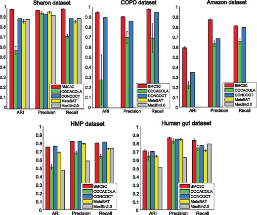
Results of BMC3C and other four binning methods (COCACOLA, CONCOCT, MetaBAT and MaxBin2.0) on five real-world datasets are shown with regards to ARI, Precision and Recall

4 Conclusions

We introduce a new computational method called BMC3C, which bins metagenomic contigs into genome bins. To reveal underlying complex structure of the datasets and to reduce the impact of noise, BMC3C performs k-means with different initializations multiple times and utilizes these k-means clustering results to build a weight graph for ensemble clustering. It subsequently employs a classical graph partitioning technique to partition the graph into subgraphs each representing a genome bin. We conduct extensive experiments on two simulated datasets and five real-world dataset to evaluate the performance of BMC3C, with reference to other related state-of-the-art binning methods. Results from these analyses consistently show that BMC3C significantly outperforms COCACOLA, CONCOCT, MetaBAT and MaxBin2.0. BMC3C presents a new paradigm to bin contigs, and this paradigm is flexible, it can also work with other clustering methods, including Gaussian mixture model and NMF. As a result, BMC3C can synergy the advantages of these base clustering methods, and neutralize or even avoid the disadvantages of them. BMC3C is also the first binning method that makes use of codon usage features, and analyses based on simulated datasets show that these features further improve the binning outcome. While BMC3C is an ensemble method, it is among the most efficient binning methods. In its current version, BMC3C does not explicitly differentiate the quality of base clusterings, and a future goal is to develop strategies to selectively integrate multiple base clusterings to further improve the performance of this method.

Funding

This work was supported by World-Class Biology Discipline of Southwest University, Natural Science Foundation of China (No. 61741217 and 61402378), Open Research Project of The Hubei Key Laboratory of Intelligent Geo-Information Processing (KLIGIP-2017A05), Natural Science Foundation of CQ CSTC (cstc2016jcyjA0351) and Hong Kong Research Grants Council Area of Excellence Scheme (AoE/M-403/16).

Conflict of Interest: none declared.

Author notes

The authors wish it to be known that Guoxian Yu and Yuan Jiang authors contributed equally.