


Abstract
The de Bruijn graph is fundamental to the analysis of next generation sequencing data and so, as datasets of DNA reads grow rapidly, it becomes more important to represent de Bruijn graphs compactly while still supporting fast assembly. Previous implementations of compact de Bruijn graphs have not supported node or edge deletion, however, which is important for pruning spurious elements from the graph.
Belazzougui et al. (2016b) recently proposed a compact and fully dynamic representation, which supports exact membership queries and insertions and deletions of both nodes and edges. In this paper, we give a practical implementation of their data structure, supporting exact membership queries and fully dynamic edge operations, as well as limited support for dynamic node operations. We demonstrate experimentally that its performance is comparable to that of state-of-the-art implementations based on Bloom filters.
Our source-code is publicly available at https://github.com/csirac/dynamicDBG under an open-source license.
1 Introduction
The de Bruijn graph was first introduced in the context of bioinformatics by Idury and Waterman (1995) and was later applied to the context of genome assembly by Pevzner et al. (2001). Since this initial application, the de Bruijn graph has become ubiquitous in the assembly and analysis of next generation sequencing data. More formally, in the edge-centric kth-order de Bruijn for a set of reads, the nodes are the set of all (k – 1)-mers in the reads and there is an edge from node u to node v if and only if there is a k-mer in the reads with prefix u and suffix v. Short-read assemblers typically use the Eulerian approach to find contiguous sequences (contigs) in the genome. Some assemblers use a single value of k, such as ABySS (Simpson et al., 2009) and Velvet (Zerbino and Birney, 2008), while other use several values of k in turn, such as IDBA (Peng et al., 2010) and SPAdes (Bankevich et al., 2012). Aside from assembly, de Bruijn graphs are also used for error correction of sequence data (Salmela and Rivals, 2014) and variant discovery (Iqbal et al., 2012).
Due to their widespread use and the large size of modern datasets, it is important that we use compact representations of de Bruijn graphs that can still be built quickly and support fast operations. Several authors have proposed representations built on Bloom filters (Bloom, 1970), which is a space-efficient probabilistic data structure built on multiple hash functions that are used to test whether an element is in a set, with the possibility of false positives. For example, Pell et al. (2012) store each k-mer in a Bloom filter, enabling the graph to be constructed and represented in 4 bits per k-mer but not with exact accuracy. This inexactness introduces false edges and branching. To ameliorate this shortcoming, Chikhi and Rizk (2013) encoded the de Bruijn graph using a Bloom Filter and an additional data structure that detects false positives. Even with this addition, they are able to assemble a human genome using 5.7 GB of memory. Salikhov et al. (2014) introduce the concept of ‘cascading Bloom filters’ that also enable false positive detection and demonstrate that they are able to reduce the memory usage by 30–40% [in comparison to Chikhi and Rizk (2013)]. In 2015, Holley et al. (2015) released the Bloom Filter Trie, which is another succinct data structure for the colored de Bruiin graph, which is a variant of the traditional de Bruijn graph.
By their nature, inserting an element into a Bloom filter is usually fairly easy since it requires only the setting of a few bits; however, deleting an element is more difficult. Moreover, compact representations of de Bruijn graphs seldom allow for easy insertions. The exceptions to this are the data structures of Belazzougui et al. (2016a) and Belazzougui et al. (2016b), which both support insertions and deletions of nodes and edges. The first is based on an extension by Bowe et al. (2012) of FM-indexes (Ferragina and Manzini, 2005) [which was further extended by Boucher et al. (2015)] and stores a pointer-based representation of recently updated nodes and edges that is incorporated into the main representation through periodic rebuilding. The second is based on a combination of Karp-Rabin hashing (Karp and Rabin, 1987) and minimal perfect hashing (Hagerup and Tholey, 2001), and supports exact membership queries. It is not clear that a complete implementation of either of these data structures would be practical but, fortunately, the second data structure becomes much simpler if we concern ourselves primarily with exact membership queries and insertions and deletions of edges. In particular, edge deletions are interesting because sequencing errors give rise to spurious nodes and edges, which are often useful to remove before assembly. Node deletions can be simulated by edge deletions, by removing all the edges incident to a node and considering that isolated nodes are effectively deleted.
In this paper, we implement the simple version of Belazzougui et al.’s hash-based data structure mentioned above, together with limited support for node insertion and removal, and we demonstrate experimentally that its performance is comparable to that of state-of-the-art implementations based on Bloom filters; in addition to the support of dynamic edge operations, our implementation efficiently supports small numbers of dynamic node operations. In Section 3 we review Belazzougui et al.’s design. We describe our implementation in Section 4, and the results of our experiments in Section 5.
2 Related work
In the previous section, we briefly discussed Bloom filter data structures for constructing and storing de Bruijn graph. Another direction is to represent the graph using succinct data structures, which is a data structure that uses an amount of space that is bounded closely to the theoretical minimum. Conway and Bromage (2011) gave a lower bound for the number of bits required to store a de Bruin graph, and then proposed a succinct data structure using bitmaps. Bowe et al. (2012) proposed a succinct representation based upon Burrows-Wheeler transforms (Burrows and Wheeler, 1994), and showed the de Bruijn graph can be represented in 4m + o(m) bits where m being the number of edges. Boucher et al. (2015) augmented this data structure to build a representation that for a given value of K constructs all th-order de Bruijn graphs, where , using only twice the space needed to construct the Kth-order de Bruijn graph. This data structure of Bowe et al. (2012) is combined with ideas from IDBA (Peng et al., 2010) in a metagenomics assembler called MEGAHIT (Li et al., 2015). Chikhi et al. (2014) implemented the de Bruijn graph using an FM-index and minimizers. Most recently, Belazzougui et al. (2016a) also extend the work of Bowe et al. (2012) in order to allow for efficient node and edge insertions and deletions. SplitMEM (Marcus et al., 2014) is a related algorithm to create a colored de Bruijn graph from a set of suffix trees representing the other genomes.
3 Algorithm
Belazzougui et al.’s data structure for a kth-order de Bruijn graph G is most-easily described in layers. At the base is a Karp-Rabin hash function that accepts either a (k – 1)-mer and returns an integer hash value in time, or accepts a (k – 1)-mer v, its hash value and a character c, and returns in time the hash value of the (k – 1)-mer obtained from v by deleting its first character and appending c (or, symmetrically, deleting its last character and prepending c). Storing this function takes asymptotically negligible space.
The next level of the data structure is a minimal perfect hash function that in -time maps integers to values in , where n is the number of nodes in G. We note that the minimal perfect hash function is bijective when restricted to the Karp-Rabin hash values of the nodes in G. Storing this function takes bits, where Σ is the alphabet (i.e. in this paper). The construction algorithm is Las-Vegas randomized: any function it returns has these properties and with high probability it returns a function in O(kn)-time with the probability taken over the random bits.
To support insertions and deletions of nodes as well as of edges, one option would be to use a dynamic minimal perfect hash function. This would require more space than a static minimal perfect hash function and the construction algorithm can return a faulty function with low probability. Therefore, in order to provide dynamic node functionality, we supplemented the static minimal perfect hash function with a binary search tree mapping (k – 1)-mers to hash values. When the number of dynamic node operations is small, say n∕1000, this scheme does not significantly increase the space occupancy of the hash function; if the binary search tree requires about 42 bytes of overhead per element inserted, in total the hash function would have increased by 0.33 bits per node after n∕1000 insertions. Hence, we denote the composition of the minimal perfect hash function and the Karp-Rabin hash function as . We note that once we have computed f(v) for a node v in G, we can compute f(w) in -time for any neighbour w of v.
The third layer is a pair of n-by-Σ binary arrays IN and OUT that indicate which incoming and outgoing edges are incident to each node. If f(v) = i then if and only if there is an edge to v from a node that starts with the (j + 1)st character in the alphabet; symmetrically, if and only if there is an edge from v to a node that ends with the (j + 1)st character in the alphabet. Each array takes |Σ| bits per node, so 4n bits in total in this paper.
Next, suppose v and w are (k – 1)-mers such that f(v) = i, v starts with the lexicographically (j + 1)st character in the alphabet, , w ends with the lexicographically st character in the alphabet, and the last k – 2 characters in v are the first k – 2 characters of w. Belazzougui et al. showed that, if and then either both v and w are in G or neither are. That is, assuming either v or w is in G, if and then the edge (v, w) is also in G. Of course, if either or then the edge (v, w) is not in G.
Using IN and OUT, if we start at a node v we think is in G then we can explore its entire connected component in the underlying undirected graph (i.e. all the nodes from which v is reachable in G and all the nodes which can be reached from v). If we encounter a discrepancy between IN and OUT—i.e. an edge (u, w) that IN says is incident to w but OUT says is not incident to u, or vice versa—then we can deduce that v was in fact not in G. Unfortunately, the absence of such a discrepancy does not confirm that v is in G.
To be able to verify whether nodes are in G, Belazzougui et al. use a fourth layer, consisting of a forest of shallow rooted trees. The edges in this forest are a subset of the edges in the undirected graph underlying G. We choose the trees to have minimum size of and maximum height of , except that we allow a tree to be smaller than when it covers an entire connected component in the underlying undirected graph. We store a binary search tree to map from the hash values of roots to their (k – 1)-mer values, mark the numbers between 0 and to which f maps those (k – 1)-mers and, for each non-root node v, we mark the edge incident to v that leads to v’s parent in the forest (To mark the requisite edges and hash values for the forest, we store bits per node.). Altogether the third and fourth layers take bits, so 13n bits in this paper, plus possibly bits for each connected component in the underlying undirected graph.
Given a node v, if f(v) is marked as being the hash value of a root, then we can check in time whether v is in G by first looking up the (k – 1)-mer corresponding to f(v) using binary search and comparing it to the (k – 1)-mer of v. Otherwise, we assume v is in G, follow the edge to its parent u (checking there is no discrepancy between IN and OUT), and check that u is in G. If v really is in G, then in time we reach the root and verify it, thus also verify v (and all its ancestors). If v is not in G, then either we will take too many steps trying to reach a root, or we will find a discrepancy between IN and OUT along the way, or when we reach a root we will find the (k – 1)-mer we are trying to check there is not the one we have stored.
If we insert an edge between two nodes in the same connected component of the underlying undirected graph, or insert an edge between two connected components each larger than , or delete an edge that is not in the forest, then we can simply update IN and OUT without updating the forest. Updating the forest when an edge is inserted between two connected components, at least one of which is smaller than , or when an edge in the forest is deleted, is the most complicated part of the data structure. Since we cannot summarize this layer quickly, we leave its full description to Section 4, where we give the details of our implementation.
The bounds for this data structure are summarized in the following theorem:
Theorem 1. Given a kth-order -ary de Bruijn graph G with n nodes, with high probability in expected time we can store G in bits plus bits for each connected component in the underlying undirected graph, such that checking whether a node is in G takes on average time, listing the edges incident to a node we are visiting takes time, crossing an edge takes time, and inserting or deleting an edge takes on average time. If at most nodes are added or removed from the data structure, then adding or removing an isolated node takes on average time, and the space occupancy does not significantly increase.
Specific Differences from Belazzougui et al. (2016b). The most significant divergence from Belazzougui et al. (2016b) is our use of a static minimal perfect hash function rather than the dynamic one proposed in the Belazzougui paper; to support limited hash changes, we supplement this static hash function with a binary search tree to map (k – 1)-mers to hash values. In addition, i) each node stores an extra bit to indicate if it is a tree root, which improves the time required to identify a root at the cost of 1 bit per node, and ii) the mapping of hash values of tree roots to (k – 1)-mers is stored in a binary search tree, which results in an additional factor whenever access to the set of root (k – 1)-mers is desired; how to store these roots was not addressed in Belazzougui et al. (2016b).
4 Implementation
Next, we give the implementation details of the dynamic data structure that we described in the previous section. In particular, the data structure is composed of the following: a hash function f that maps (k – 1)-mers to where n is the number of nodes in the de Bruijn graph, the matrices IN and OUT that encode the edges of the de Bruijn graph, and a forest covering the nodes of the de Bruijn graph. We describe the construction of each of these in Sections 4.1 to 4.3. In addition, our implementation allows for exact membership queries and vertex, edge removal and addition, which are described in Sections 4.4 and 4.5, respectively.
4.1 Hash function
The data structure relies upon a hash function f to map (k – 1)-mers to where n is the number of nodes in the de Bruijn graph. Let N be the set of (k – 1)-mers from the input reads. The hash function in our implementation is a composition g that is bijective on N, where g is a Karp-Rabin hash function (Karp and Rabin, 1987) that is injective on N, and h is a minimal perfect hash function (Hagerup and Tholey, 2001) on g(N). We next provide definitions of Karp-Rabin and minimal perfect hash functions.
Definition 1. (Karp-Rabin) Suppose we have a subset S of the universe U of all possible strings of length k over an alphabet . Given a prime P and base , a Karp-Rabin hash function g is a function defined over U such that .
Definition 2. Minimal perfect hash A minimal perfect hash function h for a set of size n, S, is a function defined on the universe such that h is one-to-one on S and the range is .
First, we discuss the procedure to generate the Karp-Rabin hash function g; the minimal perfect hash function h is then constructed using the computed Karp-Rabin values. The prime P is chosen to be the smallest prime greater than in order to give a high probability of injectivity. Next, r is chosen from a uniform distribution on 0 to ; after choosing r, we have a valid candidate for function g. The powers of and are precomputed; to compute , it is necessary to employ the generalized Euclidean algorithm. Next, g is tested for injectivity. The above process repeats with increasing primes until g is injective. After g has been generated, the minimal perfect hash h on the image of g is constructed using the library BBHash (Limasset et al., 2017). After this construction, the image of g is discarded, and only the precomputed powers of , the value of , prime P itself and g are stored.
The hash value of (k – 1)-mer may be found by first computing the sum using the stored powers of r, which can be done in O(k) time. Once the Karp-Rabin value g(a) is computed, we use the perfect hash function h to find . In the case that we have the Karp-Rabin value of a (k – 1)-mer that is a neighbor of a in the de Bruijn graph, then we can update the value of and get g(a) in O(1) time. For example, suppose is an out neighbor of a, i.e. . Then . Similarly, if is an in neighbor of a, , then .
4.1.1 Limited support for dynamic nodes
In order to allow for node insertions and deletions, a map is added on top of the minimum perfect hash function described above. The map takes (k – 1)-mers added after the initial construction of the graph to their hash value. Whenever the hash value of a kmer is computed, the map is first checked for a hash value before falling back upon the minimum perfect hash function.
When a (k – 1)-mer is added, we assign it hash value m + 1, where m is the maximum value previously assigned to any kmer. If a (k – 1)-mer is deleted from the graph, we delete the kmer from the new nodes map if it was a newly added kmer. Otherwise, no modifications are made to the hash function.
4.2 IN and OUT
The edges of the de Bruijn graph G are stored in two binary matrices, IN and OUT, each having n rows and four columns. The rows correspond to (k – 1)-mers, while the columns correspond to letters A, G, T and C, respectively.
To construct IN and OUT, first all k-mers are extracted from the input reads; IN and OUT are initialized to 0. For each k-mer, which represents an edge in the de Bruijn graph, we compute the hash value of the prefix (k – 1)-mer and then use the hash value update described in Section 4.1 in order to find the hash value of the suffix (k – 1)-mer. The corresponding entries of IN and OUT are then updated to 1. This process takes O(km) time where m is the number of edges in the de Bruijn graph. Notice that an improvement on the construction time could be made if the (k – 1)-mers were read in order of their appearance in each input read, since the hash value update could be used for all but the first (k – 1)-mer in each read.
4.3 Forest
In this section we summarize the procedure to construct the forest, which is a division of the directed de Bruijn graph into undirected trees of bounded height, where only the (k – 1)-mer of the root of each tree is stored. In our implementation is 4, and hence the tree heights are bounded by and the minimum size of a tree is α, where .
The forest is constructed within a single Breadth-First-Search (BFS) through the undirected graph underlying the de Bruijn graph. The following process is performed for each connected component. We first choose a starting node for the BFS, s, in the component. s is set as a root in the forest, and its (k – 1)-mer is stored. As we visit each node n, we set n’s parent in the forest to be its parent in the BFS by storing the following 3 bits: 1 bit to indicate whether the parent is accessed via IN or OUT, and 2 bits to indicate which of the 4 letters labels the edge to the parent. In addition, we store 1 bit to indicate whether n is a root in the forest or not.
In order to ensure that every tree has a height in the appropriate range, we also store new roots as we go along using the following process. For each node n in the component, we define a node r(n) that is an ancestor of n in the BFS representing the root of the forest tree that n is in; initially, r(n) = s for all n, and a newly discovered node in the BFS is assigned the same r as its parent. In addition, for each node n, we record the distance d(n) from n to r(n). Once we have reached a node that is of distance greater than from , we set and ; that is, we remember as a potential root and start measuring distance to in the nodes below in the BFS. Once we have reached a node n that is of distance α from r(n), we store r(n) as a root.
This way, both the new tree with root and the tree we have broken off from are both of height at least α and at most ; since a tree of height α contains at least α nodes, this procedure ensures the minimum size of each tree as well. The only exception is if a connected component is of smaller size than α; in this case, a single tree is created by the above procedure that spans the connected component. The time complexity of this procedure is . Figure 1 illustrates the forest creation procedure.
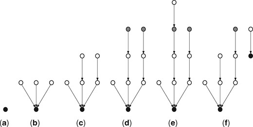
Illustration of the forest creation procedure, with α = 1. The black nodes are roots in the forest and the gray nodes are potential roots. An edge from node a to node b represents node b being the parent of node a. In stage (d), the gray nodes are at a height of , and so are potential roots. In stage (e), the furthest node from the root is at a height of , and so the potential root is stored in the forest, forming a new tree as shown in stage (f)
4.4 Membership query
Given a (k – 1)-mer x, one can query the data structure for membership of x in the nodes of the de Bruijn graph. We describe the implementation of this membership query in this section.
Whether a (k – 1)-mer x is a member of the data structure can be found by traveling up towards a root in the forest. First, we hash x, and we find the node in the forest corresponding to this hash value. Using the data stored for that forest node and x’s (k – 1)-mer, the parent’s (supposed) (k – 1)-mer is computed. The parent’s hash value is then found by using the hash update procedure described in Section 4.1. We then verify that such an edge exists between the two (k – 1)-mers in the de Bruijn graph by checking IN and OUT. If x, the (k – 1)-mer that we are querying for membership, is not a (k – 1)-mer in the graph, it may be the case that IN and OUT contradict the existence of an edge between the nodes. We can therefore eliminate the possibility of membership for some (k – 1)-mers and return false through this check. While the above test has not failed, we repeat the process with the parent’s (k – 1)-mer until we have reached a forest root or we have moved up times, that being the maximum tree height. In the latter case, the membership of x is returned false. Otherwise, if a root is reached, the (k – 1)-mer of the root computed from traveling up the tree can be compared to the stored (k – 1)-mer of the root. In this case, whether x is a member depends on whether the two are equal. An illustration of the membership query procedure can be found in Figure 2.
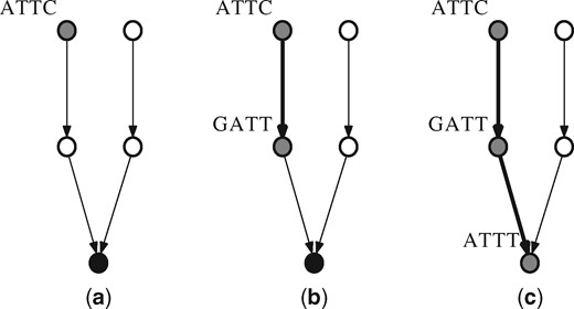
Illustration of membership query procedure for (k – 1)-mer ‘ATTC’. ‘ATTC’ is first hashed to find the corresponding node in the forest. Using the data stored for that node, it is determined that the ‘ATTC’ node has parent along an out edge with letter ‘G’. The data in OUT for the hashed value of ‘GATT’ is confirmed for a 1 for letter ‘C’. The procedure continues for ‘GATT’ and so on, until finally reaching a node which is a root and has its (k – 1)-mer stored. The membership of ‘ATTC’ is then determined by comparing ‘ATTT’ with the stored (k – 1)-mer
4.5 Updating
The data structure is dynamic with respect to edge addition and removal. In this section, we describe the procedure for updating the data structure. Both edge addition and edge removal use a tree merging procedure, which we describe first. As in previous sections, σ is 4 and we define .
4.5.1 Merge trees procedure
The merge trees procedure takes as input an ordered pair of (k – 1)-mers (u, v) such that edge (u, v) or (v, u) is in the de Bruijn graph and merges their respective trees Tu, Tv into a single tree. The procedure to merge the trees works as follows. First, we hash both u and v in time. We then reverse all of the forest edges from u to its root ru in time, ensuring that all of Tu is below u. Next, we unstore ru as a root in time. Finally, we update the forest edge of u to ensure that its parent is v in time. So in total, this procedure requires time. An illustration of the merge trees procedure can be found in Figure 3.
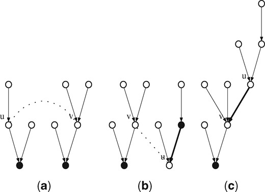
Illustration of the merge trees procedure with input nodes u and v (a). In (b), the single forest edge on the path from u to the root is reversed, so that all nodes in u’s tree can travel up to it. In (c) the root of u’s tree is unstored and v is set as u’s parent
4.5.2 Edge addition procedure
When an edge (u, v) is added between two (k – 1)-mers, we hash both u and v in time and update IN and OUT in time. Suppose u belongs to tree Tu and v belongs to tree Tv. First, we check whether either of the trees is below the minimum size in time. If neither Tu nor Tv is below the minimum size, or if Tu = Tv, the procedure exits since no update to the forest is necessary. Otherwise, suppose both Tu and Tv are below the minimum size α. In this case, the merge trees procedure is called with input (u, v). If exactly one of the trees is below the minimum size, let be the nodes corresponding to the smaller, larger trees, respectively. We compute the depth of l in its tree in time. Then, if the depth of l is at most , we simply call the merge trees procedure with pair (s, l), and the smaller tree is merged into the larger. Finally, consider the case where the depth of l exceeds . We simply travel up α steps from l in time, and store that node as a root in time. We then call merge trees for (s, l), and the smaller tree is merged into the new tree created in which l has depth α. This procedure requires a total of time.
4.5.3 Edge removal procedure
The edge removal procedure takes as input edge (u, v) to be deleted from the de Bruijn graph. First, we hash u and v in time and update IN and OUT in time. Next, we check the forest edges of u, v to see if one contains the other as its parent in its tree in time. If so, the forest is modified as follows. First, the child node is stored as a root in time, breaking off its subtree as a new tree in the forest. We then look at the trees Tp containing the former parent; we check if Tp is below the minimum size α in time. If it is, we examine each node x in Tp and look for an edge in the de Bruijn graph that is incident with both x and Tx, a tree such that , in time. If a tree Tx is found, let such that edge (x, y) or (y, x) is in the de Bruijn graph. Then the merge trees procedure is called with pair (x, y) to merge Tp into Tx. However, the resulting tree may violate the height constraint, so we check the depth dx of x in in time. Then, we find the deepest node below x in (there are at most α nodes to check). If the deepest node below x is of depth greater than , we create a new tree by traveling up steps from the deepest node and breaking off the subtree below the resulting node by storing it as a root in time. After this is done, the tree containing p has been fixed so that, if possible, the minimum size and maximum height conditions are satisfied. Finally, the tree Tc containing c is checked to see if it is below the minimum size in time, and if it is, exactly the same procedure as above is run with Tc. The procedure requires a total of time.
4.5.4 Node addition procedure
The node addition procedure takes in the (k – 1)-mer to be added to the de Bruijn graph. First, the hash function is updated as described in Section 4.1. New rows (8 bits total) are added to the end of IN and OUT in amortized time, and 4 bits corresponding to the new node are added to the forest in time. In addition, the node is initially an isolated component, and therefore its (k – 1)-mer is stored as a forest root in time.
4.5.5 Node removal procedure
The node removal procedure takes in a (k – 1)-mer already in the graph. First, each edge intersecting with the node is removed using the edge removal procedure described in Section 4.5 in time. The (k – 1)-mer then corresponds to an isolated node in the forest, which is next unstored as a forest root. Finally, the hash function is updated as described in Section 4.1. The bits corresponding to the node in IN and OUT, the forest, and the initial static hash function remain in the data structure.
5 Experiments
In this section, we evaluate that our implementation (FDBG) in comparison with reference implementations of Bloom Filter Trie (BFT) (Holley et al., 2015) and the data structure (BOSS) of Bowe et al. (2012). All data structures are evaluated in terms of construction time, final size and query time. FDBG is shown to be faster but larger than BOSS and slower but smaller than BFT.
The data structures are evaluated using read data from E. coli K-12 substr. MG1655, consisting of 27 million paired-end 100 sequence reads (NCBI SRA accession ERA000206) generated from an Illumina Genome Analyzer II. To create datasets of varying sizes, we partitioned the read data into disjoint sets of reads. For each dataset, the columns of Table 1 show the number of nodes in the de Bruijn graph and the size in bits per node of each constructed data structure.
Sizes of each data structure
| BOSS | BFT | FDBG | |
|---|---|---|---|
| 93K | 5.7 | 60.4 | 16.6 |
| 370K | 5.5 | 55.0 | 16.5 |
| 1.5M | 5.4 | 50.5 | 16.5 |
| 5.4M | 5.1 | 48.6 | 16.4 |
| 18M | 4.8 | 47.8 | 16.2 |
| 66M | 5.1 | 47.0 | 16.2 |
| 210M | 5.3 | 45.4 | 16.1 |
| 860M | 5.3 | 44.8 | 16.2 |
| BOSS | BFT | FDBG | |
|---|---|---|---|
| 93K | 5.7 | 60.4 | 16.6 |
| 370K | 5.5 | 55.0 | 16.5 |
| 1.5M | 5.4 | 50.5 | 16.5 |
| 5.4M | 5.1 | 48.6 | 16.4 |
| 18M | 4.8 | 47.8 | 16.2 |
| 66M | 5.1 | 47.0 | 16.2 |
| 210M | 5.3 | 45.4 | 16.1 |
| 860M | 5.3 | 44.8 | 16.2 |
Note: For each dataset, the columns of Table 1 show the number of unique 27-mers and the size of each constructed data structure in bits per node.
To construct the de Bruijn graph, we set k = 28. We performed all evaluations on a server with Intel(R) Xeon(R) CPU E5-2680 v2 @ 2.80 GHz and 256 GB RAM.
5.1 Construction time and space
Figure 4a shows the time required to construct each data structure, while the final size of each data structure is shown in Table 1. In our evaluation, the construction time of FDBG is comparable with the time required for BFT and BOSS and scales linearly with the number of 27-mers, as predicted by the discussion before Theorem 1. The main bottleneck for FDBG construction is the creation of the forest, which requires a depth-first search of the graph; this depth-first search also requires all k-mers to be loaded into memory; hence, more engineering on this step could improve both the memory and time required for construction of FDBG.
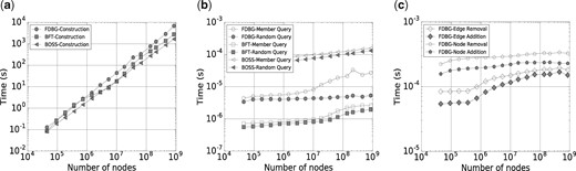
(a) Construction time (s). (b) Mean time (s) for membership queries. (c) Mean time (s) for changes to the FDBG data structure
As shown in Table 1, the final data structure of FDBG requires roughly 3 times the space of BOSS and less than 1/3 the space of BFT. The memory required by FDBG scales linearly with the number of 27-mers, also in agreement with Theorem 1. In practice, our implementation takes 13 bits per node (an extra bit is stored to indicated whether each node is a root) in addition to the space required for BBHash (Limasset et al., 2017); across all tests, BBHash required at most 4 bits per node, which yields the practical bits per node required by our implementation of FDBG.
5.2 Membership query time
Next, we evaluate the average time required for each data structure to answer membership queries: whether 27-mer u is present in the de Bruijn graph. First, we generated 106 random 27-mers and show the mean query time in Figure 4b (Random Query)—the mean query time of FDBG is slower than BFT, it is an order of magnitude faster than BOSS and remains on the order of microseconds as the number of 27-mers in the graph increases. However, since these 27-mers were generated uniformly randomly, most of these 27-mers were not in the de Bruijn graph. Often, FDBG is able to detect that a 27-mer is not a member of the graph without a full tree traversal up to the root.
A second test of the mean query time was performed where each 27-mer is selected randomly from the set of 27-mers known to be in the graph. For FDBG, each one of these queries requires a full tree traversal to the root node. Results are shown in Figure 4b (Member Query). As expected, member queries take longer than random queries, for each data structure. However, even on the largest graph tested, the average time for querying a 27-mer in FDBG is at most a few tens of microseconds and is still much faster than BOSS.
5.3 Edge deletion and addition
In order to evaluate the dynamic aspect of our data structure, we report the average time required for an edge or vertex removal and addition to the FDBG data structure, as shown in Figure 4c.
For edge removal, 50 000 edges originally present in the de Bruijn graph were uniformly randomly selected for removal. After an edge is removed, the forest is updated as described above. After all edges were removed, we reinserted all removed edges back into the de Bruijn graph. For node removal, we followed a similar procedure: a node is randomly selected for removal; before removal, all of its incident edges are removed. Then, we added the removed nodes (with incident edges) back into the data structure. The time required to update the data structure is drastically lower than the time required to construct the structure from scratch, always by more than three orders of magnitude.
6 Conclusion and future directions
In this paper, we presented a succinct de Bruijn graph representation that allows for insertion and deletion of nodes and edges. Our experiments demonstrate that FDBG requires significantly less memory than competing dynamic de Bruijn graph representations (BFT), and has efficient construction and query time. Lastly, we believe the development of dynamic de Bruijn graphs suggests future application updating a graph directly from data streaming. This would bypass the need from downloading large datasets but opens the door to other problems–such as querying public datasets to determine when to update a stored graph.
Acknowledgements
Many thanks to Simon Puglisi for suggesting this work, to Djamal Belazzougui and Guillaume Rizk for helpful discussions, and to the reviewers for their comments and suggestions.
Funding
This work was supported by the National Science Foundation [1618814] and FONDECYT [1171058].
Conflict of Interest: none declared.
References
Author notes
The authors wish it to be known that, in their opinion, the Victoria G. Crawford and Alan Kuhnle authors should be regarded as Joint First Authors.

