GWASinlps: non-local prior based iterative SNP selection tool for genome-wide association studies

Abstract

Motivation

Multiple marker analysis of the genome-wide association study (GWAS) data has gained ample attention in recent years. However, because of the ultra high-dimensionality of GWAS data, such analysis is challenging. Frequently used penalized regression methods often lead to large number of false positives, whereas Bayesian methods are computationally very expensive. Motivated to ameliorate these issues simultaneously, we consider the novel approach of using non-local priors in an iterative variable selection framework.

Results

We develop a variable selection method, named, iterative non-local prior based selection for GWAS, or GWASinlps, that combines, in an iterative variable selection framework, the computational efficiency of the screen-and-select approach based on some association learning and the parsimonious uncertainty quantification provided by the use of non-local priors. The hallmark of our method is the introduction of ‘structured screen-and-select’ strategy, that considers hierarchical screening, which is not only based on response-predictor associations, but also based on response-response associations and concatenates variable selection within that hierarchy. Extensive simulation studies with single nucleotide polymorphisms having realistic linkage disequilibrium structures demonstrate the advantages of our computationally efficient method compared to several frequentist and Bayesian variable selection methods, in terms of true positive rate, false discovery rate, mean squared error and effect size estimation error. Further, we provide empirical power analysis useful for study design. Finally, a real GWAS data application was considered with human height as phenotype.

Availability and implementation

An R-package for implementing the GWASinlps method is available at https://cran.r-project.org/web/packages/GWASinlps/index.html.

Supplementary information

Supplementary data are available at Bioinformatics online.

1 Introduction

We consider analysis of genome-wide association study (GWAS) data using variable selection regression. Majority of the frequentist and Bayesian variable selection methods, that have been applied to GWAS data (Carbonetto and Stephens, 2012; Cho et al., 2010; Guan and Stephens, 2011; He and Lin, 2011; Li et al., 2011; Wu et al., 2009) are, in theory or in implementation or in both, privileged to handle only moderate to high-dimensional data. Because GWAS data are ultrahigh-dimensional, GWAS analysis using such methods may be statistically inappropriate, often resulting in a large number of false positives, or especially for the Bayesian methods, computationally quite expensive if not infeasible. This article introduces a novel Bayesian method, which aims to ameliorate the above issues by providing efficient and parsimonious variable selection for GWAS.

A GWAS is an examination of the genetic variants, typically single nucleotide polymorphisms (SNPs), across whole genomes of different individuals. The number of SNPs measured in a GWAS may range from thousands to millions, and is much larger than the sample size. In this work, by ‘high-dimensional data’ we generally mean data where the number of independent variables, p, is one or several orders of magnitude higher than the number of samples, n and by ‘ultra-high-dimensional data’ we specifically refer to cases where the order of p is more than the polynomial order in n, i.e. $p>\mathcal{O}\left(n^c\right)$⁠. In GWAS data the number of SNPs p is often $>\mathcal{O}\left(n^c\right)$ and even $\mathcal{O}\left(c^n\right)$⁠, i.e. exponential order in n. To date, the most common approach to analyze GWAS data is single marker analysis, where individual SNPs are tested for association with a phenotype independently of the other SNPs (Zeng et al., 2015). However, such ‘single SNP analysis’ often suffer from low accountability for the total estimated heritability (the ‘missing heritability’ problem), low detection power for individual effect sizes, large number of false positives and highly conservative Bonferroni multiple comparison corrections (Gao et al., 2010; Manolio et al., 2009; Stringer et al., 2011). Contrasted to single-SNP analysis, the approach of analyzing multiple or genome-wide SNPs simultaneously has gained ample attention in the recent years, because: (i) SNPs may be correlated amongst themselves, (ii) some causal SNPs might affect the phenotype, not marginally, but only in presence of certain other SNPs and (iii) some non-causal SNPs might affect the phenotype marginally, but not when certain other SNPs are in the model (Visscher et al., 2012). However, because of the ultra-high-dimensionality of the GWAS data and higher chance of encountering correlated predictors, joint association analysis of multiple SNPs is challenging. Possible ways to handle multiple SNPs include SNP-set analysis (Wu et al., 2010, 2011) and dimension reduction through variable selection, of which the latter one is our present focus.

The most common approach to perform multiple SNP regression analysis of GWAS data is to use some form of penalized regression method. Generally, these methods add a penalty term to the cost function, forcing certain effect sizes to be set as zero and hence provide a SNP selection. Various frequentist penalized regressions methods have been used to analyze GWAS data, such as, Ridge (Whittaker et al., 2000), LASSO (Wu et al., 2009), Elastic Net (Cho et al., 2010) and adaptive LASSO (Sampson et al., 2013). Further, for ultra-high-dimensional variable selection, Fan and Lv (2008) proposed an iterative method ISIS, that takes a two-step approach to selection: first eliciting a low-dimensional subset of all predictors using some association criterion with the response, called the screening step and then selecting from that screened set of predictors using some regularized regression method, called the selection step.

In the Bayesian framework, available multi-SNP analysis methods include, but are not limited to, Bayesian LASSO (Li et al., 2011), fully Bayesian variable selection regression with Markov chain Monte Carlo (MCMC)-based inference (Guan and Stephens, 2011), Bayesian variable selection regression with variational inference (Carbonetto and Stephens, 2012), evolutionary stochastic search (Bottolo and Richardson, 2010; Bottolo et al., 2013) and Bayesian efficient linear mixed modeling (Zhou et al., 2013). All the above Bayesian methods are based on traditionally used ‘local’ priors, in contrast to which, non-local priors are recently proposed in the literature (Johnson and Rossell, 2010). In a variable (SNP) selection problem, the null value of the parameter (effect size of a SNP) associated with a predictor is typically zero, meaning that if the estimated value of the parameter deviates from the null value, the predictor is included in the model. In this context, a non-local prior on a parameter is a prior that has zero density at the null value of the parameter, whereas local priors have a positive density at the null value. It is well known that non-local priors provide parsimonious variable selection leading to reduced false positives (Johnson and Rossell, 2012). Hence, their use holds considerable promise for GWAS data analysis. Recently, Chekouo et al. (2016) have used non-local priors in the modeling of imaging genetics data with low dimension. However, direct implementation of non-local priors to high-dimensional GWAS data is computationally challenging. To the best of our knowledge, no attempt has been made to accommodate the use of non-local priors for GWAS data analysis except for the recent work by Nikooienejad et al. (2016), who developed a non-local prior based variable selection method for high-dimensional genomic studies with binary phenotypes.

In this article, we propose a novel high-dimensional variable selection method for continuous phenotypes, which is computationally efficient and provides parsimonious variable selection, making it a desirable method for GWAS data analysis. Specifically, our approach has two novelties–

• We propose an iterative scheme of variable selection, where within each iteration, variable selection is nested within a ‘structured screening’ framework. In other words, our method considers an iterative ‘structured screen-and-select strategy’ for variable selection.

• We consider the use of non-local priors within the above-mentioned structured screen-and-select framework, for analyzing GWAS data with continuous phenotypes.

The proposed iterative structured screen-and-select strategy has two intuitive advantages: first, opposed to selecting all the SNPs in one step, it breaks down the selection problem into small chunks thereby making small or moderately high-dimensional methods applicable within each chunk and secondly, it performs screening hierarchically through the imposition of a structure that is informed by the dependence pattern in the data. On the other hand, for linear models, specifically non-local prior based procedures achieve model selection consistency for $p\le \mathcal{O}\left(n\right)$⁠, whereas local prior based procedures have not been shown to have this consistency and frequentist model selection procedures including the penalized likelihood-based methods are shown to have such consistency when p is fixed a priori or $p\le \mathcal{O}\left(n^{1/3}\right)$ (Johnson and Rossell, 2012). Hence, the use of non-local priors to select variables within our structured-screen-and-select framework is an appealing choice. As the implementation of non-local prior based variable selection for small to moderately high-dimensional linear models is fast, endowed with the above advantages, our method is able to provide an efficient and parsimonious variable selection for GWAS with continuous phenotypes. We call our method iterative non-local prior based selection for GWAS, or GWASinlps, which is described in the following section.

2 Materials and methods

2.1 Phenotype model

Let us consider n subjects, each having genotype values for p SNPs. Suppose ${\mathbf{y}}^{n\times 1}=(y_1,y_2,\dots ,y_n)$ is the vector of continuous phenotypes (such as height, weight, blood pressure), and ${\mathbf{X}}^{n\times p}$ is the matrix of genotype values, henceforth called the genotype matrix, with ith row x_i corresponding to subject i. The genotype value for subject i and SNP j is the number of a particular reference allele (most often the minor allele) of SNP j, present in subject i. We consider biallelic SNPs and an additive genetic model. Hence, the genotype values are 0, 1, or 2. Suppose ${\mathit{\beta }}^{p\times 1}=\left({\beta }_1{,\beta }_2{,\dots ,\beta }_p\right)$ denotes a regression vector of SNP effect sizes.

In the variable (or model) selection context, a collection of SNPs defines a model. With p SNPs, we can have 2^p distinct models. Let us index a model by $\mathbf{k}=\{k_1,k_2,\dots ,k_j\}$⁠, with $1\le k_1<k_2<\dots <k_j\le p$⁠, and assume that for model $\mathbf{k}$⁠, the vector of SNP effects is ${\mathit{\beta }=\mathit{\beta }}_{\mathbf{k}}$ with ${\beta }_{k_1},{\beta }_{k_2},\dots ,{\beta }_{k_j}\ne 0$ and ${\beta }_{k\prime }=0$ for all $k\prime \in \{1,2,\dots ,p\}\setminus \{k_1,k_2,\dots ,k_j\}$⁠, where $j\in \{0,1,\dots ,p\}$⁠. Further suppose ${\mathbf{X}}_{\mathbf{k}}$ denotes the design matrix corresponding to model k and ${\mathbf{x}}_{i\mathbf{k}}$ denotes the ith row of ${\mathbf{X}}_{\mathbf{k}}$⁠. With these notations set, for model k, we assume that the ith response y_i arises from a general linear model, given by

$$y_i={\mathbf{x}}_{i\mathbf{k}}^{\prime }{\mathit{\beta }}_{\mathbf{k}}+{ϵ}_i,$$

(1)

where ${ϵ}_i,i=1,\dots ,n$⁠, are identically and independently distributed normal errors with mean 0 and unknown variance ${\sigma }_{ϵ}^2$⁠. Note that, if there are other available covariates (such as age, gender, principal components), which may be considered as confounding variables, they can be included in the ${\mathbf{X}}_{\mathbf{k}}$ matrix as well. Alternatively, one can adjust the phenotype vector and individual SNP genotype vectors for these confounders by updating these vectors with residuals from univariate regressions with the confounders as predictors (Price et al., 2006). For visual simplicity, we do not use explicit notations for the confounders here.

2.2 Non-local priors for SNP effect sizes

For the SNP effects vector ${\mathit{\beta }}_{\mathbf{k}}$⁠, in contrast to traditionally used local priors, we consider a non-local prior (Johnson and Rossell, 2010), that converges to zero as the effect size tends to its null value, which is typically 0 in the variable selection context. In this work, we investigate two choices of the non-local prior for the effect sizes––the product moment prior (pMOM prior) and the product inverse moment prior (piMOM prior; Johnson and Rossell, 2012). For model k, in what follows, let us denote the non-zero elements of ${\mathit{\beta }}_{\mathbf{k}}$ by $({\beta }_{1\mathbf{k}},{\beta }_{2\mathbf{k}},\dots ,{\beta }_{\left|\mathbf{k}\right|\mathbf{k}})$⁠, where $\left|\mathbf{k}\right|$ is the number of SNPs included in model k.

As the first choice, for the non-zero components of ${\mathit{\beta }}_{\mathbf{k}}$ we assume a pMOM prior, which is the product of individual moment (MOM) priors on those non-zero components, and can be expressed as

$$\pi ({\mathit{\beta }}_{\mathbf{k}}\hspace{0.17em}|\hspace{0.17em}r,{\tau ,\sigma }^2)=M_{\left|\mathbf{k}\right|}^{-1}{\left({\tau \sigma }^2\right)}^{-\frac{\left|\mathbf{k}\right|}{2}-r\left|\mathbf{k}\right|}\prod _{k=1}^{\left|\mathbf{k}\right|}{\beta }_{i\mathbf{k}}^{2r}\hspace{0.17em}\text{exp}\hspace{0.17em}\left[-\sum _{k=1}^{\left|\mathbf{k}\right|}\frac{{\beta }_{i\left|\mathbf{k}\right|}^2}{2{\tau \sigma }^2}\right],$$

(2)

where $M_{\left|\mathbf{k}\right|}={(2\pi )}^{-\left|\mathbf{k}\right|/2}{\left((2r-1)!!\right)}^{\left|\mathbf{k}\right|}$⁠, with $(2r-1)!!={\prod }_{j=1}^r(2j-1)$⁠, is a marginalizing constant independent of τ and r, $r=1,2,\dots$ is the order of the prior, τ > 0 is a scale parameter and ${\sigma }^2={\sigma }_{ϵ}^2$⁠.

As the second choice, for the non-zero components of ${\mathit{\beta }}_{\mathbf{k}}$ we assume a piMOM prior, which is the product of individual inverse moment (iMOM) priors on those non-zero components, and can be expressed as

$$\pi ({\mathit{\beta }}_{\mathbf{k}}\hspace{0.17em}|\hspace{0.17em}\nu ,{\tau ,\sigma }^2)=\frac{{\left({\tau \sigma }^2\right)}^{\frac{\nu \left|\mathbf{k}\right|}{2}}}{{(\Gamma (\frac{\nu }{2}\left)\right)}^{\left|\mathbf{k}\right|}}\prod _{k=1}^{\left|\mathbf{k}\right|}|{\beta }_{i\mathbf{k}}{|}^{-(\nu +1)}\hspace{0.17em}\text{exp}\hspace{0.17em}\left[-\sum _{k=1}^{\left|\mathbf{k}\right|}\frac{{\tau \sigma }^2}{{\beta }_{i\left|\mathbf{k}\right|}^2}\right],$$

(3)

where ν  >  0 and τ  >  0 are, respectively, the shape and the scale parameters of the prior, and σ² is defined similarly as for the pMOM prior.

Figure 1 depicts the density curves of the MOM (r = 1, τ  =  1) and iMOM (ν  =  1, τ  =  1) priors in red and blue solid lines, respectively. The construction of the MOM prior is based on Normal density (red dashed line) whereas the iMOM prior is functionally related to the inverse gamma density (blue dashed line). Consequently, the MOM prior has tail behavior similar to the Normal distribution, whereas the iMOM prior has heavier tails. On the other hand, in the vicinity of zero, iMOM prior vanishes quite rapidly compared to the MOM prior. Intuitively these imply: (i) if a standardized effect size is large, the iMOM prior, by virtue of possessing heavier tails, allows greater support for its detection and unbiased estimation, whereas the MOM prior might over-shrink, leading to bias; (ii) if a standardized effect size is small (but non-zero), the MOM prior provides better support for its detection and unbiased estimation, whereas iMOM prior might lead to bias from over-shrinking. Because of this trade-off, the usefulness of the choice of non-local prior will depend on the nature of the effect size distribution of the data under consideration.

Fig. 1.

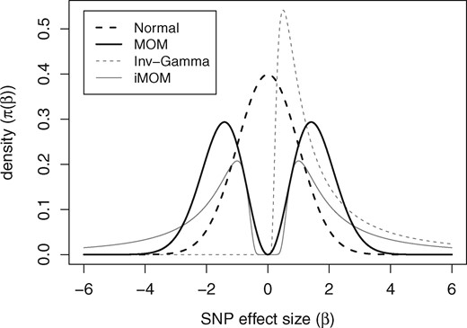
MOM prior (r = 1, τ  =  1) and iMOM prior (ν  =  1, τ  =  1) in solid lines; N(0, 1) and the Inv-Gamma (1, 1) distributions in dashed lines

Note that, in the expressions of the priors for the effect sizes, if only one component of the effect size vector ${\mathit{\beta }}_{\mathbf{k}}$ is zero, the density $\pi \left({\mathit{\beta }}_{\mathbf{k}}\right)$ is zero. This is a crucial feature of the pMOM and piMOM priors, which imposes, for variable selection, a strong penalty on the regression vector with at least one 0 component, facilitating consistent identification of the causal SNPs (Johnson and Rossell, 2012) and for coefficient estimation, a strong data-dependent shrinkage on the effect sizes (Rossell and Telesca, 2017). Following Johnson and Rossell (2012) we assume an inverse gamma (0.01, 0.01) prior for ${\sigma }_{ϵ}^2$⁠, and a beta-binomial prior for the model space, given by $\pi \left(\mathbf{k}\right|\gamma )={\gamma }^{\left|\mathbf{k}\right|}\hspace{0.17em}{(1-\gamma )}^{p-\left|\mathbf{k}\right|}, \text{with} \gamma \sim \text{beta} (1,1)$⁠.

2.2.1 Choice of hyperparameters

For simplicity, we set r = 1 for the pMOM prior and ν  =  1 for the piMOM prior. In fact, for r ≥ 2 the MOM prior becomes considerably peaked on both sides of zero followed by a rapid fall to zero while the tail behavior stays similar. Hence, considering r > 1 may lead to increased bias. The other hyperparameter τ, for both the priors, controls how much dispersed the prior is around 0. The larger τ is, the more well-spread is the prior over the parameter space and so relatively large values of the parameter are encouraged. However, a smaller τ is more likely to detect the effect of smaller values of the parameter. As GWAS effect sizes are generally very small, in this work, we estimate τ such that the non-local prior assigns a probability of 0.01 to the event that a standardized effect size will fall in the interval (–0.05, 0.05). Such estimates of τ for the MOM and iMOM priors are 0.022 and 0.008, respectively (Johnson and Rossell, 2010).

2.3 GWASinlps method

The GWASinlps method is designed to select SNPs iteratively in steps. Given an initial list of SNPs, S, the genotype matrix X and the phenotype vector y, the procedure begins in iteration 1 by determining those k₀ SNPs that have highest ranking in association with the phenotype. We refer to these k₀ SNPs as the leading SNPs of the iteration. Absolute value of the Pearson correlation coefficient between a SNP and the phenotype is considered as the measure of association. The association measures are computed based on the pairwise-complete data points. Suppose $S_1,S_2,\dots ,S_{k_0}$ denote the k₀ leading SNPs that are determined by the association ranking.

For each leading SNP $S_j,j=1,\dots ,k_0$⁠, independently of others, we determine all those SNPs (including S_j) that have absolute correlation coefficients with S_j more than or equal to r_xx, where r_xx ∈ (0, 1) is a given threshold. Conceptually this amounts to determining all those SNPs that are in LD with S_j with a strength at least r_xx. Let ${\mathbf{S}}_j=(S_{j1},S_{j2},\dots ,S_{j{l}_j})$ denote the set of all such SNPs. We call ${\mathbf{S}}_j,j=1,2,\dots ,k_0$⁠, the leading sets of the iteration. Determination of the leading SNPs and subsequent determination of the leading sets, combinedly, constitute a ‘structured screening’ procedure, which is an innovative approach in the literature of variable selection based on the ‘screen-and-select’ strategy and has important consequences for our GWASinlps method as discussed in the Discussion Section.

For each leading set ${\mathbf{S}}_j,j=1,\dots ,k_0$⁠, we perform non-local prior-based Bayesian variable selection only with the SNPs included in S_j (Johnson and Rossell, 2012). The Bayesian variable selection is based on the phenotype model specified in Equation (1), the non-local prior for the SNP effect sizes specified in Equation (2) or Equation (3) and the specified model space prior. Specifically, the variable selection is achieved by generating MCMC simulations from the posterior distribution on the model space, identifying the model with the highest frequency of appearance among the simulations as the HPPM and then selecting the SNPs included in the HPPM. Suppose ${\mathbf{S}}_j^{\text{sel}}$ is the set of selected SNPs from the leading set ${\mathbf{S}}_j$⁠.

Define ${\mathbf{S}}_{\left(1\right)}=\underset{j=1}{\overset{k_0}{\cup }}{\mathbf{S}}_j$ as the set of all SNPs from all leading sets S_js and ${\mathbf{S}}_{\left(1\right)}^{\text{sel}}=\underset{j=1}{\overset{k_0}{\cup }}{\mathbf{S}}_j^{\text{sel}}$ as the set of all selected SNPs from all S_js. We consider ${\mathbf{S}}_{\left(1\right)}^{\text{sel}}$ as the set of SNPs selected at iteration 1. The SNPs in ${\mathbf{S}}_{\left(1\right)}$ are dropped from the initial SNP list. In addition, the response vector y is updated with the residuals from a multiple regression of y on the SNPs in ${\mathbf{S}}_{\left(1\right)}^{\text{sel}}$⁠.

With the updated list of SNPs and the updated response vector from iteration 1, iteration 2 proceeds similarly as above. Provided the updated SNP list contains at least one SNP, the procedure may continue selecting SNPs through successive iterations until a pre-determined number m of selected SNPs is reached and m determines a stopping criterion. In any iteration i, if ${\mathbf{S}}_{\left(i\right)}^{\text{sel}}$ is empty, we remove the SNPs in ${\mathbf{S}}_{\left(i\right)}$ from S, skip the rest of the ith iteration and jump to the (i + 1)th iteration. The maximum allowed count of such skipping, denoted by n_skip, determines another stopping criterion of GWASinlps.

Together with all the constraints, the GWASinlps procedure is outlined in Algorithm 1. One essential feature of GWASinlps is that, within an iteration, a SNP that is correlated with multiple leading SNPs has opportunity to be selected from multiple non-local prior based MCMC runs on multiple leading sets. So, even if a SNP is not selected from one leading set, it may well be selected from some other leading set. However, if a SNP, present in one or more of the leading sets, is not selected in the current iteration altogether, that SNP is dropped from subsequent iterations. As such, GWASinlps provides an elegant trade-off between two extremes–dropping a SNP immediately if it is not selected at one instance, at one hand, and giving a SNP indefinite consideration for getting selected, on the other. It is advisable to use imputed data as input in the GWASinlps procedure as the non-local prior based Bayesian variable selection requires fully available design matrix.

Algorithm 1

GWASinlps procedure

Require:$\mathbf{S},\hspace{0.17em}\mathbf{X},\mathbf{y},\text{family},k,r_{xx},m,n_{\text{skip}}$

1: $i\leftarrow 0,\hspace{0.17em}skip\leftarrow 0,\hspace{0.17em}{\mathbf{S}}^{\text{sel}}\leftarrow []$

2: while$\mathbf{c}\mathbf{a}\mathbf{r}\mathbf{d}({\mathbf{S}}^{\text{sel}})<m$and$\mathbf{c}\mathbf{a}\mathbf{r}\mathbf{d}(\mathbf{S})>0$andskip$<n_{\text{skip}}$do

3:  $i\leftarrow i+1$

4:  $S_1,S_2,\dots ,S_{k_0}$$\leftarrow$ (Leading SNPs) Top k₀ SNPs in $\mathbf{S}$ with highest absolute correlation, $|$cor(⁠$\mathbf{X}[‘S_j’],\hspace{0.17em}\mathbf{y}$⁠)$|$⁠, with $\mathbf{y}$

5:  forj = 1 to k₀do

6:   ${\mathbf{S}}_j\leftarrow (S_{j1},S_{j2},\dots ,S_{j{l}_j})$$\leftarrow$ (Leading set) All SNPs with absolute correlation $\ge r_{xx}$ with S_j

7:   ${\mathbf{S}}_j^{\text{sel}}$$\leftarrow$ SNPs in the HPPM obtained from non-local prior based variable selection within S_j

8:  end for

9:  ${\mathbf{S}}_{(i)}\leftarrow \underset{j=1}{\overset{k_0}{\cup }}{\mathbf{S}}_j,\hspace{0.17em}{\mathbf{S}}_{(i)}^{\text{sel}}\leftarrow \underset{j=1}{\overset{k_0}{\cup }}{\mathbf{S}}_j^{\text{sel}}$

10:  if${\mathbf{S}}_{(i)}^{\text{sel}}$ is non-empty then

11:   ${\mathbf{S}}^{\text{sel}}$$\leftarrow$$[{\mathbf{S}}^{\text{sel}},{\mathbf{S}}_{(i)}^{\text{sel}}]$

12:   $\mathbf{y}$$\leftarrow$ Residuals from multiple regression of $\mathbf{y}$ on the SNPs in ${\mathbf{S}}_{(i)}^{\text{sel}}$

13:  else

14:   skip$\leftarrow$skip + 1

15:  end if

16:  $\mathbf{S}\leftarrow \mathbf{S}\setminus {\mathbf{S}}_{(i)}$

17:  $i\leftarrow i+1$

18: end while

19: return${\mathbf{S}}^{\text{sel}}$

2.3.1 Choice of GWASinlps tuning parameters

GWASinlps has several tuning parameters, namely, k₀, r_xx, m, n_skip, that should be chosen considering prior knowledge on the dataset and/or experimenter necessity. Regarding k₀, setting a low value will maintain a low number of leading sets, and consequently some causal SNPs that affect the phenotype better only in presence of certain other SNPs may not get selected, but such setting will safeguard against false positives. However, if the dataset contains only a few SNPs with high association measure with the phenotype, unless their effects are removed, other causal SNPs may not get selected and in that case, choosing a large k₀ may just increase the computational time without any gain in detection.

The intuitive choice of r_xx is 0.5. However, in the genetics literature, for an LD-pruned GWAS dataset, an inter-SNP correlation of 0.2 may often be considered high enough, especially if the SNPs belong to the same chromosome. Hence, a reasonable choice of r_xx should depend on the application specific need and background. However, for a GWAS dataset that has not been LD-pruned, the leading sets will generally be much larger in size and the evaluation of HPPM will be computationally costing without giving much gain. Hence, for unpruned datasets a higher value of r_xx is recommended.

We may let GWASinlps procedure to continue running until no SNP is left to become a leading SNP. Alternatively, given constraints in terms of m and/or n_skip, the stopping point is determined by whichever constraint is challenged first. Here, we arbitrarily set n_skip = 3 and m = 500, a large number.

2.3.2 Prediction

After GWASinlps-based SNP selection, the selected SNPs may be used in an estimation model to perform effect size estimation and phenotype prediction. For the applications in the simulated and real data studies discussed below, we use a non-local prior based estimation model (Rossell and Telesca, 2017) that considers the full model regressing the phenotype on all the GWASinlps selected SNPs, and generates samples from the posterior distribution of the SNP effect sizes. The SNP effect sizes are estimated using the mean of these posterior samples. Finally, the predicted values of the phenotype are obtained by using these effect size estimates in Equation (1).

2.4 Simulation studies

In order to demonstrate the performance, flexibility and advantage of the GWASinlps method, we conduct extensive simulation study with SNPs having realistic LD structure. We divide all the simulations into two sets: Simulation 1, used to perform methods comparison and Simulation 2, used to perform power analysis.

2.4.1 Simulated data for methods comparison (simulation 1)

In simulation 1, for methods comparison we considered analysis of simulated data with SNP genotypes having an LD structure resembling that of real genotyped SNPs. We varied both the number of SNPs p and the number of samples n and for each combination of p and n, independently generated datasets. Specifically, we considered three different values for both p and n. Corresponding genotype matrices were generated using HAPGEN2 (Su et al., 2011) as follows. From the SNPs present in chromosome 1 p-arm, we constructed three sets: SNPs belonging to region 3 (bp 1–84 400 000), regions 2 and 3 (bp 1–106 700 000) and regions 1, 2 and 3 (bp 1–123 400 000). In each set, we retained only those SNPs that are included in the legend files of the phased haplotypes from the HapMap 3 release 2 (see Supplementary Material Web Resources). Next, using the SNPs of each set in HAPGEN2, for three different sample sizes 2000, 3000 and 5000, we generated genotype matrices having similar LD structure as the chromosome 1 haplotypes present in the CEU+TSI reference panel and similar fine-scale recombination rates as in the genetic map of chromosome 1. The generated genotype matrices were randomly pruned using a reference LD matrix of ∼9 million SNPs and a threshold of r² = 0.8 (Wang et al., 2016). Regular quality control was performed using 0.01 minor allele frequency (MAF) threshold. Duplicate SNP columns and constant SNP columns were removed. After the above steps, the number of SNPs in the three sets was approximately 10 000, 15 000 and 20 000, which are the three different values of p considered for the analysis. For each SNP set, we randomly chose 20 SNPs as the causal SNPs. For the causal SNPs, standardized effect sizes were independently generated from the N(0, 1) distribution. For the remaining SNPs, the effect sizes were set as zero. In order to generate the phenotype data, we considered five heritability values 0.1, 0.2, 0.3, 0.4 and 0.5. Phenotypic variance explained (PVE) was considered to represent heritability. Thus, for a given heritability h², the phenotypes were generated by adding to $\mathbf{X}\mathit{\beta }$⁠, independent N(0, SD  =  η) noise, where η was determined such that $h^2=\text{var}(\mathbf{X}\mathit{\beta })/\left(\text{var}\right(\mathbf{X}\mathit{\beta })+\eta ).$ For each combination of p and n, we simulated 100 independent replicates.

2.4.2 Simulated data for power analysis (simulation 2)

In simulation 2, to conduct power analysis for our GWASinlps method we considered, as before, simulated SNP genotypes with realistic LD structure. The genotype matrix was generated using HAPGEN2 (Su et al., 2011) in the following way. We selected all chromosome 21 SNPs contained in the legend files of the phased haplotypes from the HapMap 3 release 2 (c.f. Simulation 1). The number of selected SNPs were 19 306. We considered 19 different sample sizes ranging from n = 1000 to n = 10000, increasing by 500. For each sample size, using the selected SNPs in HAPGEN2, we generated genotype matrix having similar LD structure as the chromosome 21 haplotypes present in the CEU+TSI reference panel, and similar fine-scale recombination rates as in the genetic map of chromosome 21. Similarly to Simulation 1, the generated genotype matrices were randomly pruned, subjected to regular MAF correction and corrected for duplicate and constant SNP columns. After the above steps, ∼8000 SNPs were left in the genotype matrices of all sample sizes. From the SNPs common to all genotype matrices, we randomly selected 25 SNPs as causal SNPs. For the causal SNPs, standardized effect sizes were independently generated from the N(0, 1) distribution. For the remaining SNPs, the effect sizes were set as zero. To generate the phenotype data, we considered three heritability values 0.05, 0.1 and 0.15. Representing heritability by PVE, for a given heritability h², the phenotypes were generated by adding to $\mathbf{X}\mathit{\beta }$⁠, independent N(0, SD  =  η) noise, where η was determined similarly as in Simulation 1. For each combination of p and n, 100 independent replicates were simulated.

2.5 Thematically organized psychosis data

We applied our GWASinlps method to analyze a real dataset obtained in the Norwegian Thematically Organized Psychosis (TOP) research study at the University of Oslo and Oslo University Hospital (see Supplementary Material Web Resources). The dataset contains imputed genotype data from three different batches for controls and patients diagnosed with severe mental illness. As recent research showed that human height is considerably polygenic in nature (Yang et al., 2010), we considered height as the phenotype in our analysis. The genotype data from the several different batches were combined, and the combined data underwent regular quality control whereby SNPs with MAF less than 0.01 were removed and LD-based pruning with a threshold of r² = 0.8 (c.f. Simulation 1). Further, if duplicate SNPs columns were present, only one was retained and any all-equal SNP column was removed. The number of retained SNPs was ∼55 000. We adjusted the values of height and SNP genotypes for gender by updating them with the residuals from univariate regression on gender.

2.6 Implementation and scalability

We have implemented our GWASinlps method within the programming language R (R Core Team, 2016). We used the following R packages: mombf (Rossell et al., 2016) for non-local prior computations, glmnet (Friedman et al., 2010) for regularized regression analysis and snowfall (Knaus, 2015) for parallel programming to facilitate computation. The software pi-MASS was used to implement the analysis of Guan and Stephens (2011). All parallel computations were performed using the Extreme Science and Engineering Discovery Environment, supported by National Science Foundation grant number ACI-1053575 (Towns et al., 2014). The genetic simulation software HAPGEN2 (Su et al., 2011) was used to simulate genotype matrices. LD-pruning was performed using the commercial software package MATLAB (MATLAB, 2016). We wrote an R package implementing our method and made it freely available.

Regarding scalability and speed, GWASinlps breaks up the whole selection problem into small chunks by means of a structured screening that needs to compute only the Pearson’s correlation coefficients between variables. Within each small chunk, Bayesian variable selection is a low-dimensional to at most a moderately high-dimensional problem (⁠$p\le \mathcal{O}(n\hspace{0.17em}\text{log}(n\left)\right)$⁠). As computation of Pearson’s correlation is of $\mathcal{O}\left(n\right)$ complexity and very fast using R (and most other standard softwares), with proper choices of the tuning parameters k₀ and r_xx, handling ultrahigh-dimensional data is computationally efficient for our method when compared to relevant existing methods and does not present any advanced level of challenge.

3 Results

In this section, we present the results from the simulated and real data analyses. The statistics that we have used for the evaluation of the variable selection and prediction are (i) true positive rate (TPR) or sensitivity (the number of causal SNPs selected divided by the number of causal SNPs), (ii) false discovery rate (FDR; the number of non-causal SNPs selected divided by the number of SNPs selected), (iii) mean squared error (MSE) of prediction, (iv) l₂ estimation error in the effect sizes (⁠$\mathit{\beta }$-error) and (v) relative prediction gain (RPG; Guan and Stephens, 2011), which is a unitless number that measures how much of the extractable signal present in the data has been detected by a method and is defined as

$$\text{RPG}=\frac{ \text{MSE} \text{using} \text{only} \text{intercept}-\text{MSE} \text{using} \text{estimated} \text{effect} \text{sizes} }{ \text{MSE} \text{using} \text{only} \text{intercept}-\text{MSE} \text{using} \text{true} \text{effect} \text{sizes} }.$$

Thus, if the PVE (heritability) of a phenotype is 0.1, then an RPG of 0.6 for a method indicates that the method can extract 60% of this PVE from the data, which is to say, the method can explain 6% of the total variance in the phenotype values.

3.1 Simulation 1 analysis results

In Simulation 1 analysis, we compare our GWASinlps method with frequentist LASSO (Tibshirani, 1996) and Elastic net (Zou and Hastie, 2005) methods and Bayesian pi-MASS (Guan and Stephens, 2011) method. In addition, we compare GWASinlps results with the results obtained using Zellner’s g-prior (Zellner, 1986) within our structured screen-and-select framework instead of a non-local prior, henceforth referred to as igps.

We analyzed Simulation 1 datasets using GWASinlps (⁠$k_0=1,r_{xx}=0.2$⁠) with pMOM and piMOM priors and also using igps (⁠$k_0=1,r_{xx}=0.2$⁠) with frequently used setting g = n, LASSO and Elastic Net with tuning parameter α  =  0.75, 0.5, 0.25 and pi-MASS. For LASSO and Elastic Net, two mostly used choices of the tuning parameter λ were considered: the value of λ that gives minimum mean cross validated error, henceforth called l.min and the largest value λ such that error is within 1 standard error of the minimum, henceforth called l.1se, both in a 10-fold cross validation. For GWASinlps analysis, we used 1800 MCMC iterations after 200 burn-ins, whereas for pi-MASS we used 10 000 iterations after 1000 burn-ins.

We average the Simulation 1 analyses results across the considered heritability values, and in what follows, present these average measures. For a real GWAS data, n and p will be known but true h² will generally not be known, so it is meaningful to compare method performances averaged across the unknown quantity. However, we make the heritability-specific individual estimates available in the Supplementary Tables S1 through 5. We summarize the results of Simulation 1 analyses in Figure 2 showing barplots of TPR and FDR, and Figure 3 showing barplots of MSE and $\mathit{\beta }$-error. We note that, LASSO with l.1se tuning performed better than l.min tuning in all cases. So, for clarity, in these figures we show only l.1se based results. Both figures constitute of nine cells arranged in a three-by-three grid with number of SNPs in rows and number of samples in columns. Specifically, each cell in Figure 2 shows the barplots of TPR (in darker shade) and FDR (in lighter shade) for several different competing methods. On the other hand, each cell in Figure 3 shows barplots of MSE (in denser lines) as percentage of the highest observed MSE in all (n, p) combinations, and barplots of $\mathit{\beta }$-error (in sparser lines) as percentage of the highest observed $\mathit{\beta }$-error in all (n, p) combinations, for all the competing methods. Because of the difference in the order of MSE and $\mathit{\beta }$-error, percentage measures were used to avoid distortion of the graphs, for the sake of presentation. We make the actual error estimates available in the Supplementary Tables S4 and S5.

Fig. 2.

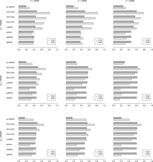
Simulation 1 barplots of TPR and FDR of variable selection for all (n, p) combinations, using our GWASinlps pMOM and piMOM methods, Zellner’s g-prior within our structured screen-and-select framework, LASSO, Elastic Net with several choices of tuning parameter α and pi-MASS. All the results are averaged across the considered heritability values and 100 replicates

Fig. 3.

Simulation 1 barplots of MSE and l₂ estimation error in effect sizes (⁠$\beta$-error) for all (n, p) combinations, using our GWASinlps pMOM and piMOM methods, Zellner’s g-prior within our structured screen-and-select framework, LASSO, Elastic Net with several choices of tuning parameter α and pi-MASS. All the results are averaged across the considered heritability values and 100 replicates, and then expressed as percentages of the highest observed value of the corresponding error in all (n, p) combinations

We note that, compared to the regularized regression methods, GWASinlps has provided (i) much lower FDR, with competing TPR uniformly across sample size and number of SNPs, (ii) almost equal TPR for larger p, i.e. in presence of higher sparsity which is usual in GWAS data and (iii) uniformly lower MSEs and $\mathit{\beta }$-errors across sample size and number of SNPs. Further, we note that, with the increase of heritability, GWASinlps yielded decreasing number of false discoveries whereas the regularized regressions methods mostly showed an increasing trend. On the other hand, pi-MASS with comparable number of MCMC iterations as GWASinlps selected too few SNPs and resulted in inferior results compared to all other methods. Note that, igps method, which enjoys our structured screen-and-select framework, has performed better than the regularized regression methods and pi-MASS, as well. This clearly demonstrates the utility and efficient model space exploration ability of our proposed structured screen-and-select approach. In Figure 2, the performance of igps is quite competitive with GWASinlps. Figure 3 shows whereas igps generally provided smaller $\mathit{\beta }$-error, GWASinlps generally provided smaller MSE, which is intuitively justified as the non-local priors achieve model selection consistency with $p=\mathcal{O}\left(n\right)$ (Johnson and Rossell, 2012). Further, we note that GWASinlps with pMOM prior has shown slightly better performance than with piMOM prior in overall analysis. Hence, for Simulation 2, we present only pMOM-based results.

Regarding computational time, average runtime for dataset with n = 2000, 3000, 5000 were respectively about 0.6 mins, 0.8 mins and 1.1 mins for pMOM prior, and 3.1 mins, 4.5 mins and 5.4 mins for piMOM prior and average runtime for dataset with p = 10 000, 15 000, 20 000 were, respectively, about 0.6 mins, 0.8 mins and 1.1 mins for pMOM prior and 5.6 mins, 3.1 mins and 4.3 mins for piMOM prior.

3.2 Simulation 2 analysis results

In Simulation 2 analysis, we perform power analysis for our GWASinlps method using both (variable) selection power and prediction power. We divided each Simulation 2 dataset into train and test data allotting three-quarters of samples to the train data. We analyzed the train datasets using our pMOM-based GWASinlps method with $k_0=1$ and r_xx = 0.2, which is a stringent setting favoring the minimization of false positives. The power of variable selection, or selection power, empirically was defined as the TPR. The power for prediction was assessed through RPG. Both estimates were averaged over the 100 independent replicates. The results of Simulation 2 analyses are presented Figure 4 showing plots of TPR, and Figure 5 showing plots of RPG. For all considered heritabilities, Figure 4 shows the evolution of selection power and the corresponding false positive count, as the sample size is increasing. In Figure 5, we show the evolution of RPG for the train and test data with increasing sample size. We note that for the lowest considered heritability 0.05, below the sample size of 3000, the RPG values showed unstable fluctuations because of overfitting. So, for the sake of better visual representation, in Figure 5, we truncated the plots below n = 3000. We make all Simulation 2 TPR, TNR, FDR and RPG values available in the Supplementary Tables S6 and S7.

Fig. 4.

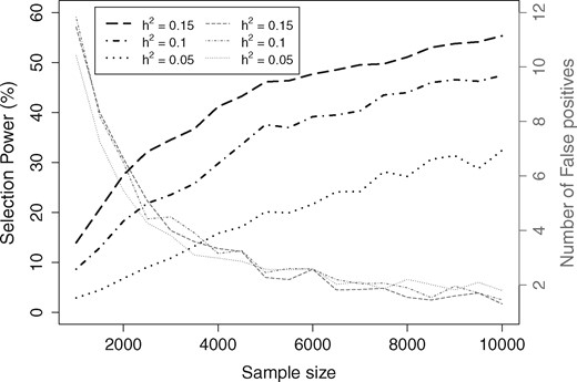
Simulation 2 plots of selection power and number of false positives for sample size varying from 2000 to 10 000 and the three considered heritability (h²) values from GWASinlps pMOM-based analysis. All the points are averaged across 100 replicates

Fig. 5.

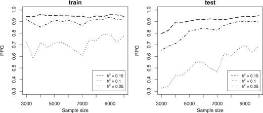
Simulation 2 plots of RPG for prediction in train and test data using GWASinlps method for sample sizes 3000 upwards and the considered heritability values. Values below n = 3000 are unstable because of overfitting and truncated for better visual representation

From Figure 4, we note that with sample size increasing, selection power has increased steadily whereas number of false positives decreased, as would be desired. Figure 5 test data plot shows that with the increase of sample size, our method has been able to detect more and more of the extractable signal present in the data. Both the figures nicely demonstrate the consistency of our variable selection method.

3.3 Sensitivity analysis for GWASinlps tuning parameters

As the GWASinlps method depends on few tuning parameters, we perform a sensitivity analysis. Unless the experimenter wishes to obtain at most a specific number of selected SNPs, m is set at a high value by default. Hence, for the sensitivity analysis, we consider the other tuning parameters k₀, r_xx and n_skip. As data, we use the first 30 replicates corresponding to p = 10 000, n = 2000 and h² = 0.5 from Simulation 1. We consider the following grid of values: $k_0\in \{1,2,3,4,5\},\hspace{0.17em}{r}_{xx}\in \{0.2,0.35,0.5,0.75,0.9\}$ and $n_{\text{skip}}\in \{1,2,3,4,5\}$⁠, which contain the specific values of the tuning parameters used in Simulations 1 and 2 analyses. We analyze the datasets using GWASinlps pMOM prior-based method with each combination of $(k_0,r_{xx},n_{\text{skip}})$ from the above grid of values.

As a measure of assessing sensitivity of the analysis to the choices of tuning parameters, we consider MSE. The MSEs from the sensitivity analysis are provided in the Supplementary Table S8. Note that, lower values of k₀ and r_xx will safeguard more against false positives, and hence will tend to yield sparser SNP selection, whereas higher values of k₀ and r_xx will tend to yield more liberal SNP selection and hence will automatically lead to lower MSEs. However, from the Supplementary Table S8, we see that the fluctuation of MSE in the whole considered grid of tuning parameters is quite modest. The range of all the MSEs is (8.23, 9.15) with a SD of 0.27, which is not very high for a sample size of n = 2000.

3.4 TOP data analysis results

To analyze the real dataset with GWASinlps, we considered 20 random divisions of the data into train and test data allotting three-fourth of the subjects to the train data. For each division, GWASinlps (⁠$k_0=1,r_{xx}=0.2$⁠) with pMOM prior was applied to the corresponding train data, resulting in a set of selected SNPs. The number of SNPs that appeared in at least half (i.e. 10) of these SNP sets is 7, whereas the number of SNPs that appeared in at least one-fourth (i.e. 5) of these SNP sets is 26. The MSEs from the train and test data are respectively 44.82 and 46.86 using the above 7 SNPs, and 40.24 and 50.98 using the above 26 SNPs. Specifically, with those 7 SNPs there is almost no overfitting. All the above 26 SNPs along with their chromosomal positions, frequency of appearance in the above twenty sets, rs IDs and gene symbols are given in Supplementary Table S9. In addition, for each of the above 20 considered divisions, we also performed variable selection using LASSO, Elastic Net and pi-MASS. No SNP was selected for any of the divisions using LASSO and Elastic Net with α varying from .01 to 1 either with l.min or l.1se based regularization. On the other hand, although pi-MASS selected few SNPs for each division, the number of common selected SNPs among all divisions was zero.

4 Discussion

We have developed a novel Bayesian method, GWASinlps, for GWAS variable selection by combining in an iterative framework, the computational efficiency of the screen-and-select approach based on some association learning and the parsimonious uncertainty quantification provided by the use of non-local priors. Although the frequently used regularized regression methods, such as LASSO and Elastic Net are able to handle high-dimensional GWAS data and when implemented through l.min based regularization provide estimates with low MSE, the number of selected SNPs is often too large, defeating the purpose of a meaningful variable selection. One frequently used alternative is to use l.1se based regularization, that produces lesser false positives (Friedman et al., 2010). In this work, through the simulation studies, we have shown that our proposed GWASinlps method is able to provide a sparser SNP selection than the above regularized regression methods by largely reducing the FDR while maintaining a highly competitive profile in terms of TPR and MSE. Simulation 1 analysis clearly shows that, in overall comparison, GWASinlps has achieved a superior balance between parsimony and predictive ability compared to both l.min and l.1se based regularized regression methods. Further, in Simulation 2, by extensive empirical power analysis, we have provided guidelines for determining adequate sample size for detecting effect sizes in various ranges and for achieving desired prediction rates, which are useful for study design.

Our method is a Bayesian adoption of the ‘screen-and-select’ approach and comparable to the similar frequentist approach ISIS (Fan and Lv, 2008). Both GWASinlps and ISIS select variables iteratively. However, there are some important differences. Within each iteration, whereas ISIS screens a pre-fixed number of predictors based on phenotype-predictor association, GWASinlps performs the screening process hierarchically in two steps, where the first step is guided by phenotype-predictor association and the second step is guided by predictor-predictor association. We call this ‘structured screening’, which is a generalization over the one-stage screening process of Fan and Lv (2008). Within each iteration, such structured screening is, what we think, the hallmark of our method and furnishes our method the ability to evaluate a SNP with respect to its ‘belongingness’ to multiple groups of SNPs. Moreover, after an iteration, whereas ISIS drops and regresses out the selected predictors of that iteration, GWASinlps drops all the screened predictors of that iteration, but only regresses out the selected predictors. The intuition is that in presence of the structured screening and the subsequent selection, such iterational dropping of predictors will reduce the redundancy in the overall selection process. In addition, compared to GWASinlps, the computational scalability of ISIS is quite inferior, for which we did not venture ISIS-based analysis of Simulation 1. In addition, with a comparatively lower number of MCMC iterations, GWASinlps selected more true causal SNPs than the fully Bayesian method pi-MASS, which becomes computationally quite costing for large number of MCMC simulations.

Although in Simulation 1, the pMOM prior has shown better performance than the piMOM prior, such may not be the case always. As discussed previously, compared to the iMOM prior, the MOM prior provides more support for the detection of smaller effect sizes. Generally, for polygenic traits the effect sizes of individual causal SNPs are low, as is the case in our simulations as well. In such situations, the pMOM prior is expected to work better. However, if the effect sizes are more dispersed, the piMOM prior might outperform the MOM prior.

Desirable extensions of the GWASinlps method may include extension for binary or categorical data analysis, and adaptation to the analysis of GWAS summary data. Although applied to GWAS data in the current work, the basic form of the GWASinlps method is generic in nature. Hence, although in this work we have set the values of the GWASinlps tuning parameters considering background information and experimenter necessity, it may be desirable to develop strategies to optimally estimate these GWASinlps tuning parameters from data.

Recently, non-local priors have been used in sparse modeling regression where the regression coefficients are assumed to arise from a mixture of a point mass and a non-local prior (Sanyal and Ferreira, 2017). Such sparse modeling framework has been applied to imaging genetics data (Chekouo et al., 2016) with low dimension. A possible extension of our current method is to make such non-local prior based sparse modeling feasible for GWAS data.

Acknowledgements

The authors would like to thank associate editor John Hancock and the three anonymous reviewers whose comments and suggestions have definitely contributed towards an improved version of the manuscript. NS developed the methods, designed the simulation studies, analyzed data and wrote the manuscript. CHC provided guidance for study design and manuscript preparation. VEJ provided guidance for method development. CHC, MTL, KK, SD and OAA helped in obtaining, processing and understanding of the TOP data. CHC, VEJ and OAA commented on the manuscript.

Funding

This work was supported by National Institute of Mental Health [R01MH100351] (NS, MTL, CHC) and National Cancer Institute [R01CA158113] (NS, VEJ) of the National Institutes of Health, and KG Jebsen Stiftelsen and Research Council of Norway [223273, 229129] (OAA, SD).

Conflict of Interest: none declared.