


Abstract
Visualizing and reconstructing cell developmental trajectories intrinsically embedded in high-dimensional expression profiles of single-cell RNA sequencing (scRNA-seq) snapshot data are computationally intriguing, but challenging.
We propose DensityPath, an algorithm allowing (i) visualization of the intrinsic structure of scRNA-seq data on an embedded 2-d space and (ii) reconstruction of an optimal cell state-transition path on the density landscape. DensityPath powerfully handles high dimensionality and heterogeneity of scRNA-seq data by (i) revealing the intrinsic structures of data, while adopting a non-linear dimension reduction algorithm, termed elastic embedding, which can preserve both local and global structures of the data; and (ii) extracting the topological features of high-density, level-set clusters from a single-cell multimodal density landscape of transcriptional heterogeneity, as the representative cell states. DensityPath reconstructs the optimal cell state-transition path by finding the geodesic minimum spanning tree of representative cell states on the density landscape, establishing a least action path with the minimum-transition-energy of cell fate decisions. We demonstrate that DensityPath can ably reconstruct complex trajectories of cell development, e.g. those with multiple bifurcating and trifurcating branches, while maintaining computational efficiency. Moreover, DensityPath has high accuracy for pseudotime calculation and branch assignment on real scRNA-seq, as well as simulated datasets. DensityPath is robust to parameter choices, as well as permutations of data.
DensityPath software is available at https://github.com/ucasdp/DensityPath.
Supplementary data are available at Bioinformatics online.
1 Introduction
Cell fate is determined by transition states which occur during complex biological processes, such as proliferation and differentiation. The recent advent of massively parallel single-cell RNA sequencing (scRNA-seq) provides snapshots of single-cell transcriptomes, thus offering an essential opportunity to unveil the molecular mechanism of cell fate decisions (Tanay and Regev, 2017; Trapnell et al., 2014). The high-dimensional cellular profiles by scRNA-seq are heterogeneous populations of cells at diverse stages of cell proliferation and differentiation, making it a computational challenge to infer the progression of cell fate decisions based on scRNA-seq data.
Researchers have dedicated extensive efforts to computationally reconstruct pseudo-trajectories of cellular development from single-cell data (Chen et al., 2018; Kumar et al., 2017). Monocle, which relied on building the minimum spanning tree (MST) on cells, pioneered the study of reconstruction of complex pseudo-trajectory for scRNA-seq data (Trapnell et al., 2014). However, Monocle is computationally intractable for large-scale data. Wanderlust, another pioneer study, attempted to construct a linear trajectory based on the k-nearest neighbor (k-NN) graph for single-cell mass cytometry data (Bendall et al., 2014). To further reveal the hierarchical structure of cell lineage, Wishbone extended the Wanderlust algorithm to construct a developmental bifurcating trajectory with two branches (Setty et al., 2016). Diffusion pseudotime (DPT) developed a diffusion distance to calculate the pseudotime, leading to reconstruction of the branched trajectory (Haghverdi et al., 2016). Although it is possible to identify lineage bifurcating event(s) for large-scale single-cell data, Wishbone and DPT only construct simple branched trajectories, restricted to two branches, or requiring the number of branches as a priori.
In order to reconstruct complex cell trajectories of cell development at affordable computational cost, methods based on embedding curve/graph techniques have been developed (Ji and Ji, 2016; Marco et al., 2014; Qiu et al., 2017; Rizvi et al., 2017). These methods fitted/mapped d-dimensional single-cell data points onto a one-dimensional curve or graph and then ordered the cells along the curve/graph to approximate the trajectory of cell development. SCUBA (Marco et al., 2014) fitted single-cell data points with the principal curve, a smooth one-dimensional curve that passes through the ‘middle’ of data points (Hastie et al., 2009). However, based on the necessity of infinite differentiation, the principal curve cannot handle self-intersecting data structure, e.g. branched trajectory (Mao et al., 2017). Thus, SCUBA had to require additional temporal information and perform the K-means algorithm on temporal windows to extract cellular lineage relationships. Tools for Single Cell Analysis (TSCAN) (Ji and Ji, 2016) used an approach that grouped cells into clusters by a hierarchical clustering algorithm, constructed an MST by connecting cluster centers, and then projected each cell onto the tree to obtain the pseudotime of cells. Single cell Topological Data Analysis (Rizvi et al., 2017) applied a topological data analysis tool called Mapper (Singh et al., 2007) to the single-cell data, intending to unveil the intrinsic topological structures of cell developmental processes. The Reeb graph constructed by single cell Topological Data Analysis included not only tree-like structures, but also loops or holes. However, these topological data analysis methods may be sensitive to data noise (Mao et al., 2017). Monocle2 (Qiu et al., 2017), a descendant of Monocle, adopted a recently developed principal graph method, termed reversed graph embedding (RGE) (Mao et al., 2017), to find the complex trajectories of single-cell data. The principal graph method handles the self-intersecting data structure by a collection of piecewise smooth curves, allowing these curves to intersect each other (Mao et al., 2017). To implement it, RGE utilized a K-means algorithm to obtain K centroids of clusters and then found the spanning tree between the centroids to construct the principal graph. However, clustering methods, such as hierarchical clustering and K-means algorithm, as applied by the methods noted above, to seek an optimal partition of the data may be unstable when the data are heterogeneous and noisy or exhibit complex multimodal structure.
Single-cell gene expression profiles by scRNA-seq are characterized by their high dimensionality. Therefore, in most algorithms that construct cell developmental trajectories, the very first, indeed, the key, step is to embed single-cell expression data onto a lower-dimensional space. Dimension reduction and visualization methods, such as principal component analysis (PCA), diffusion map (DM) and t-distributed Stochastic Neighbor Embedding (tSNE), are commonly used for scRNA-seq (Chen et al., 2018; Kumar et al., 2017). However, as pointed out by Moon et al. (2017), these methods are limited in their ability to recover the complex structures of scRNA-seq data. For example, PCA is a linear method which cannot handle non-linear structures; DM, which can learn non-linear transition paths, tends to place different branches into different diffusion dimensions, making it difficult to visualize complex trajectories with multiple branches; tSNE can reveal and emphasize the cluster structures in data, while tending to shatter trajectories and failing to preserve the global structures.
In this study, we present a novel algorithm, DensityPath (Fig. 1), allowing visualization of the intrinsic structure of scRNA-seq data on an embedded 2-d space and reconstruction of optimal cell state-transition paths of complex trajectories on the density landscape. DensityPath requires no a priori knowledge of trajectory structure (e.g. number of cell states and number of branches), while still maintaining computational efficiency and accuracy. DensityPath consists of the three major steps. First, it allows the visualization of high-dimensional gene expression profiles of scRNA-seq data by adopting the non-linear dimension reduction algorithm elastic embedding (EE) (Carreira-Perpiñán, 2010). As an extension of tSNE, EE can preserve both local and global structures of the data (Section 3.1, also see Wasserman, 2018). DensityPath constructs the density landscape of cells to visualize the intrinsic structure in a 2-d space by EE. Second, to explore and reveal the heterogeneous subpopulation structure of single-cell data, DensityPath develops a density-based method of level-set clustering (LSC) (Wasserman, 2018). The LSC scans the multi-mode density landscape and extracts the separate high-density clusters of cells, as representative cell states (RCSs), in an unsupervised manner. These identified RCSs are then used as the landmarks of the density landscape. Third, DensityPath reconstructs the cell state-transition path by finding the MST of the peak points based on their calculated geodesics on the surface of density landscape. Since the potential energy function can be defined as the negative logarithm of the probability distribution (Moon et al., 2017; Wang et al., 2011), the RCSs can be regarded as the attraction basins and their peak points can be regarded as the saddle points of the underlying interaction potential energy as in equilibrium systems. The cell state-transition path based on geodesic distance computed by DensityPath is equivalent to the optimal transition state path on the energy landscape going through the saddle points, establishing a least action path with minimum-transition-energy similar to the dominant minimum energy kinetic path in equilibrium systems (Section 3.1, also see Wang, 2015).
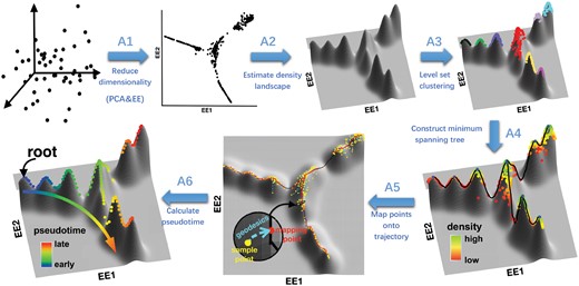
Overview of DensityPath algorithm. DensityPath offers a method to visualize and reconstruct complex cell developmental trajectories intrinsically embedded in the high-dimensional expression profiles of scRNA-seq snapshot data by a series of steps. First (step A1), using PCA and EE, it reduces the high-dimensional scRNA-seq data into a d-dimensional embedded space (d=2). Second (step A2), it estimates the density function (landscape) of single cells on the embedded space of EE1 and EE2. Third (step A3), it selects the high-density clusters of RCSs by LSC. Fourth (step A4), it constructs the cell state-transition path on the surface of density landscape by finding the MST of the peaks of RCSs based on the geodesics. Fifth (step A5), it maps the single cells onto the cell state-transition path using the geodesics on the density surface. Sixth, (step A6), it calculates the pseudotime when a start cell (root) is determined. The dot points in each plot are the single cells. See Sections 2.3 and 3.1 for details
We demonstrate that power of DensityPath in allowing the visualization and reconstruction of complex cell developmental trajectories, in particular, those with multiple bifurcating and trifurcating branches, on both real and simulated scRNA-seq datasets. Meanwhile, DensityPath presents high accuracy and efficiency in pseudotime calculation and branch assignment. DensityPath is robust in terms of parameter choices, number of informative genes, subsampling cells and dropout events.
2 Materials and methods
2.1 EE
2.2 LSC
The LSC algorithm is a density-based clustering method [see Wasserman (2018) and KIM et al. (2016) for details]. Given a collection of samples that are independently drawn from the probability distribution F with density function f, the t-upper level-set is defined as . The connected components of Lt, denoted as , are called the density clusters at level t. As shown in Supplementary Figure S1a, as t increases, the size of Lt will decrease. After t rises and crosses the valley of adjacent peaks, a connected component of Lt will be broken into two separate connected components. Then, after t rises and crosses a peak, one connected component will vanish. Finally, after t rises and crosses the highest density peak, Lt will be empty. By increasing the threshold t, LSC scans the heterogeneous multimodal density landscape, examines how density cluster breaks or vanishes at different level t on the density function, as shown in Supplementary Figure S1. Therefore, LSC represents the topological structure of the density function as a rooted hierarchical tree structure (density tree) of density clusters . Each branch therein represents a connected density cluster, and the ancestor branch splits into descendent branches at the ‘height’ where the corresponding density cluster breaks into two or more separate density clusters on the density function. Meanwhile, the external branch terminates at the ‘height’ where the corresponding density cluster vanishes (Supplementary Fig. S1b). LSC finally extracts the representative separate high-density clusters as level-set clusters of the data, which are represented by the external branches of the constructed density tree shown in Supplementary Figure S1b.
2.3 DensityPath algorithm
The flowchart of DensityPath is shown in Figure 1. The main steps for DensityPath are as follows:
A1. Reduce the dimensionality of scRNA-seq data. The DensityPath algorithm first performs PCA to map data in original space into the top principal components which preserve the most variance. The choice of dimension embedded in PCA is achieved by cutting off the ordered eigenvalues of PCA at the first i-th largest eigenvalue λi, the difference of adjacent eigenvalues of which is less than a given threshold ε, i.e. the i satisfying . We choose in this study. Following dimension reduction through PCA, DensityPath then applies the EE algorithm (Carreira-Perpiñán, 2010; Vladymyrov and Carreira-Perpiñán, 2013; Vladymyrov and Carreira-Perpiñán, 2012) to the top i-th largest components of PCA, embedding them into the d-dimensional latent space. We show that d = 2 is sufficient to preserve the intrinsic structures of scRNA-seq data, even for data with complex trajectory with branches both from bifurcations and trifurcations (Section 3.3). We denote the two coordinates from EE algorithm as ‘EE1’ and ‘EE2’ throughout this study.
- A2. Estimate the density function landscape. DensityPath estimates the density function (landscape) of the reduced-dimension space of single-cell expression profiles using the standard non-parametric kernel density estimator as
where is the estimated density function, H is the full bandwidth matrices for multivariate kernel density estimation, K is the Gaussian kernel (Wassermann, 2006) and n is the sample size. The choice of bandwidth H is calculated based on the ‘plug-in’ method (Sheather and Jones, 1991; Woodroofe, 1970).
A3. Select high-density clusters of RCSs by LSC. DensityPath applies the LSC method (KIM et al., 2016; Wasserman, 2018) to the density landscape estimated as to extract high-density clusters as RCSs (see details in Section 2.2). The estimated and are utilized instead. For any t > 0, the estimated t-upper level-set is calculated as . To identify the connected components of , DensityPath first constructs a k-NN graph of on the reduced-dimension space and then finds the connected components of the subgraph with the nodes restricted to the index set .
A4. Construct the cell state-transition path. DensityPath uses the peak points of RCSs as landmarks and calculates the shortest distance path (geodesic) of the peak points on the surface of the density landscape using Dijkstra’s algorithm (see Supplementary Note S1). The embedded cell state-transition path is then constructed by finding the MST of the peak points based on their calculated geodesics on the surface of density landscape.
A5. Map the single cells onto the cell state-transition path. Each cell is projected onto the cell state-transition path constructed in A4 such that the projected point has the smallest geodesic distance to the cell. The projection may be considered in the sense of orthogonality when the mapping is constrained on the surface of density landscape. All cells are placed in order according to the projected positions along the cell state-transition path.
A6. Calculate the pseudotime of each cell. For a fixed start cell (root) and any given cell, the pseudotime of the given cell is defined as the geodesic distance between projected positions of two cells (the start cell and the given cell) on the cell state-transition path.
The overview of DensityPath is found in Section 3.1; the pseudocode of DensityPath is given in Supplementary Table S2.
DensityPath has two tunable parameters. First, the regularization parameter λ of the EE algorithm in Equation (1) trades off two terms, one preserving local distance and the other preserving global distance, or separate latent points. DensityPath sets the default of λ as 10. The second involves the number of k neighbors for the k-NN graphs in LSC. The choice of k generally relies on the sample size n. Here we propose an empirical formulation to compute k as k = round(n/100), i.e. the nearest integer value of n/100. We demonstrate the robustness for the choices of λ and k in Supplementary Note S9.
2.4 Data
We test DensityPath on three real scRNA-seq datasets of mouse bone marrow cells (Paul et al., 2015) (hereinafter denoted as Paul data), mouse hematopoietic stem and progenitor cells bifurcating to myeloid and erythroid precursors (Setty et al., 2016) (hereinafter denoted as HSPCs data) and human pre-implantation embryos (Petropoulos et al., 2016) (hereinafter denoted as HPE data), as well as two simulated datasets: the simulated complex trajectory embedded data from Moon et al. (2017) (hereinafter denoted as PHATE data) and the simulated bifurcating trajectory embedded data from Zwiessele and Lawrence (2017) (hereinafter denoted as SLS3279 data). See Supplementary Note S2 for details of data availability and data pre-processing.
2.5 Method evaluations
To evaluate pseudotime calculation and branch assignment performance, we adopt Pearson’s correlation coefficient (PCC) and adjusted rand index (ARI) (Qiu et al., 2017; Rand, 1971) (see Supplementary Note S3).
3 Results
3.1 Overview of DensityPath
In this study, we present a novel algorithm, DensityPath, which allows visualization of the intrinsic structures and reconstruction of optimal cell state-transition path for large-scale scRNA-seq data (see Section 1, Fig. 1 and Section 2.3). The power of DensityPath is realized by the nature of the following procedures.
Through DensityPath, the intrinsic structure of high-dimensional gene expression profile of scRNA-seq data on an embedded intrinsic 2-d space can be visualized by applying both PCA and EE (Carreira-Perpiñán, 2010). Both tSNE and EE embed the high-dimensional data points into the stable low-dimensional latent space by modeling the data points interactively with two terms. One term attracts pairs of points toward each other, while the other term of the simultaneously repulsive force separates all pairs of points. A similar embedding idea has been adopted by force atlas embedding (Jacomy et al., 2014), which has also been recently adopted in the visualization of scRNA-seq data (Weinreb et al., 2018b). Force atlas embedding lays out the k-nearest-neighbor graphs in a manner mentioned above that preserves high-dimensional relationships and represents the graphical data on a 2-d space (Jacomy et al., 2014; Weinreb et al., 2018b). As an extension of tSNE, EE penalizes placing close together latent points from dissimilar data points in the original space (Carreira-Perpiñán, 2010) instead of the latent space, as is done by tSNE. With this improvement, as we illustrate in Section 3.3, EE preserves both local and global intrinsic data structures in the 2-d plane quite well (Wasserman, 2018). Meanwhile, since the weight of the repulsive force is defined on the original space, this improvement by EE also prevents intersecting lines between clusters that are separated in high-dimensional space, in the 2-d space.
DensityPath develops the LSC method (Wasserman, 2018) to analyze the heterogeneous multimodal behavior of the density landscape and extract high-density separate clusters as RCSs (Section 2.2). The level-set method is a mathematical tool for the numerical analysis of surfaces and shapes, and it has been successfully applied in unsupervised clustering, image processing and computational fluid dynamics, among others (Hartigan, 1975; KIM et al., 2016; Osher and Fedkiw, 2002; Wasserman, 2018). The idea behind it involves the reduction of overall data complexity by breaking complex datasets into a series of separate high-density clusters, each of which is then regarded as a representative class of data (Cadre, 2006). A comparison of LSC with other clustering methods is given in Section 4.
DensityPath takes the RCSs identified by LSC as the landmarks of the density landscape. In order to construct the transition path of the RCSs, we find that existing metrics on LSC mainly consider the ‘height’ at which two points, or two clusters, merge on the density function (KIM et al., 2016), but which is insufficient to measure the transition distance between the points, or clusters, on the density function. Therefore, in DensityPath, we propose a metric of differential geometry for RCSs. In detail, instead of using the Euclidean distance or density tree metric, DensityPath calculates the geodesic, or shortest distance path, of the single-cell points, and then finds the MST of the peak points based on their calculated geodesics on the surface of density landscape. As pointed out in the Section 1, the peaks of RCSs can be regarded as the saddle points of the underlying interaction potential energy, as in equilibrium systems. Since the optimal cell state-transition path should go along the gradient descent direction of the potential landscape passing through the saddle points when the system is in equilibrium (Wang, 2015), DensityPath therefore calculates geodesics between the peak points of RCSs and reconstructs the cell state-transition path by connecting the peak points with the MST on the surface of density landscape, aiming to approximate the least action path (dominant minimum energy kinetic path) (Wang, 2015). Each edge of the MST is connected by two peak points, passing through the intermediate low-density point of their valley in between. It will be intriguing to reconstruct trajectories on the non-equilibrium landscape (see Section 4).
With high accuracy and efficiency, we demonstrate that DensityPath visualizes and reconstructs not only simple branched trajectories on Paul data (Supplementary Note S4 and Fig. S2), HSPCs data (Supplementary Note S5 and Fig. S3) and SLS3279 data (Supplementary Note S6 and Fig. S5), but also complex trajectories with multiple bifurcating and trifurcating branches on HPE data (Section 3.2) and PHATE data (Sections 3.3 and 3.4).
3.2 DensityPath reveals cell fates of complex trajectories with both bifurcating and trifurcating events on HPE
We apply DensityPath to the HPE data of 1529 single cells of HPE from Petropoulos et al. (2016). The cells isolated from embryos, ranging from the eight-cell stage up to the time point just prior to implantation, were collected and labeled with time from embryonic day 3–7 (E3–E7). The cell differentiation process of HPE was reported as the synchronous differentiation of the inner cell mass (ICM) into three distinct cell types of the mature blastocyst: trophectoderm (TE), primitive endoderm and epiblast at E5 from the zygote (Petropoulos et al., 2016). Besides the dominant processes involving segregation of ICM, the cells in TE lineage were also reported to be further subdivided into two subpopulations, reflecting that polar and mural cells are present within the TE lineage (Petropoulos et al., 2016).
We select the 4600 most variable genes across all cells, as in Rizvi et al. (2017), for further DensityPath analysis. DensityPath constructs the density landscape of the cells on the EE coordinates (Fig. 2a), and then extracts 14 high-density clusters of RCSs with sizes ranging from 1 to 84, summing up to 500 of the total 1529 cells (Fig. 2b). DensityPath connects the peak points of RCSs by the MST on the surface of density landscape, resulting in a complex trajectory with two bifurcating events and one trifurcating event (Fig. 2b and d). Finally, DensityPath calculates the pseudotime of the cells (Fig. 2c), having a high PCC of 0.8286 with the experimental embryonic time.
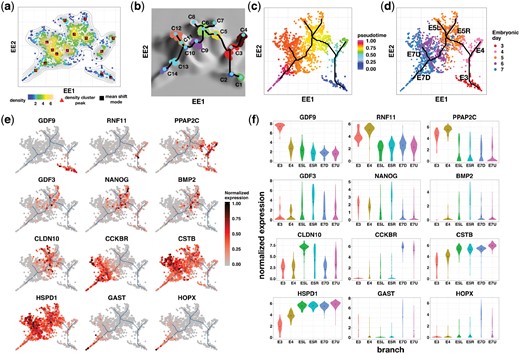
DensityPath visualizes and reconstructs the complex trajectory of HPE data. (a) DensityPath estimates the density landscape of single cells on a 2-d plane of EE. The red triangle points are the peak points of RCSs identified by DensityPath, while the black squares are the modes (local maxima) identified by the MS algorithm. (b) DensityPath reconstructs a complex trajectory with 2 bifurcating events and 1 trifurcating event by connecting the peaks of the 14 separate RCSs identified by LSC. (c) Given a start cell (cell No. 1481 in the data), DensityPath calculates the pseudotime of each cell with cell start time set as 0. (d) The cells from embryonic day 3–7 are plotted with different colors on the embedded 2-d space of EE. The branches of the cell state-transition path are annotated according to the embryonic day and their positions on the plot. For example, ‘E7U’ stands for the upside branch occurring at E7. (e) The scattering plots of genes of the cells on the embedded 2-d space of EE showing the branch-specific expression patterns. (f) The violin plots of gene expressions for cells mapped onto each branch. The branch labels ‘E3’,, ‘E7U’ correspond to the branch annotations in (d), respectively
The trifurcating event identified by DensityPath occurs among cells from E5 (Fig. 2d), which is completely consistent with the progression during E5 in which the ICM lineage separates into primitive endoderm, epiblast and ICM lineages (Petropoulos et al., 2016). The bifurcating event appearing at E6 and E7 (Fig. 2d) is also consistent with the existence of two subpopulations which occurred in the progression of the TE lineage (Petropoulos et al., 2016). In addition, we also identify a newly bifurcating event recovered at E4 (Fig. 2d), which was not reported in Petropoulos et al. (2016).
We further identify several branch-specific expressed genes (Fig. 2e and f), validating the two bifurcating and one trifurcating events reconstructed by DensityPath. The identified genes show spatial patterns of gene expression on the embedded 2-d space by EE (Fig. 2e), and by mapping the cells onto the cell state-transition path as in step A5, those genes show high expression levels at specific branches (Fig. 2f; the branches are annotated according to Fig. 2d). For example, genes RNF11 and PPAP2C are highly expressed in the cells mapped to the ‘E4’ branch (Fig. 2e and f), supporting the existence of the bifurcating event recovered at time E4.
3.3 DensityPath visualizes the intrinsic structure of scRNA-seq data in the 2-d plane
By adopting the EE algorithm for dimension reduction, DensityPath visualizes the hidden complex trajectories in the 2-d plane of EE1 and EE2, preserving the intrinsic structure, both globally and locally. We illustrate this with the simulated PHATE data from Moon et al. (2017), which contains 1440 single cells and 60 genes. The PHATE data have an embedded continuous tree structure with 10 branches, each of which contains around 140 points (cells) in different data subdimensions of a 60-dimensional space to model a system within which the progression along a branch corresponds to an increasing expression of several genes. The tree has three bifurcating events and one trifurcating event. The trunk (starting branch in red color) first bifurcates into two branches (green and black), one (green) of which subsequently bifurcates into two branches, while the other one (black) trifurcates into three branches, followed by one (blue) of the three branches further bifurcating into two branches (see the embedded tree structure in Fig. 3a, which is based on Fig. 7a of Moon et al., 2017).
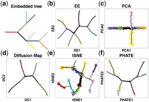
Visualization of the intrinsic structure of PHATE data by different methods. (a) Embedded tree structure of simulated PHATE data. (b) EE. (c) PCA. (d) Diffusion Map. (e) tSNE. (f) PHATE algorithm. Colors of points in (b–f) are annotated according to the branch assignments of cells in (a). The black curves in (b–f) correspond to their trajectories reconstructed according to the procedures described in steps A2–A4 of DensityPath
DensityPath maps the data onto the 2-d plane of EE1 and EE2 and reconstructs the complex trajectory with 10 branches, recovering the simulated progression of the embedded tree structure completely (Fig. 3b). In comparisons, PCA identifies four branches with one trifurcating event (Fig. 3c); DM identifies five branches with two bifurcating events (Fig. 3d); tSNE breaks the samples into at least five separate components, shattering the order of trajectory and failing to preserve the global structures (Fig. 3e). The PHATE algorithm developed by Moon et al. (2017) also recovers the simulated structure completely (Fig. 3f). However, the branch lengths on the 2-d plane by EE (Fig. 3b) are more uniformly distributed than those revealed by the PHATE algorithm (Fig. 3f), showing better consistency with uniform branch lengths of the embedded tree model.
We compare EE with the other 4 dimension reduction methods on the HSPCs data. The PCA, tSNE and EE all recover the branched trajectories (Supplementary Fig. S4), but DM fails to recover the branched structure on the first two diffusion components (Supplementary Fig. S4). The PATHE algorithm also fails to recover the branching structure in its first two components (Supplementary Fig. S4).
EE can, in general, reveal the intrinsic structure of data in 2-d space (Section 3.1). We also embed the three real datasets of Paul, HSPCs and HPE into 3-d latent space by EE. The third dimension EE3, however, does not provide additional information on distinguishing the structure of clusters (see detailed results in Supplementary Note S7 and Fig. S31).
3.4 DensityPath reconstructs optimal cell state-transition paths of complex trajectories with high accuracy
DensityPath reconstructs the optimal cell state-transition path (Section 3.1). When applied to the PHATE data, DensityPath recovers the embedded complex trajectory completely (Fig. 3b). With the initial cell fixed as the starting point of simulated time, we calculate the pseudotime of the cells and branch assignment (Supplementary Figs S12 and S13). The PCC between pseudotime recovered by DensityPath and the real time of the simulation is 0.9528, while the ARI value between the branch assignment of the cells to the reconstructed trajectory by DensityPath and the ground truth by simulation is 0.7317.
Furthermore, when we conduct systematic comparisons of DensityPath with Monocle2, DPT, Wishbone and TSCAN on Paul data, HPE data and simulated datasets of PHATE and SLS3279, we find that DensityPath outperforms other methods in terms of complex trajectory reconstruction, pseudotime calculation and branch assignment (see detailed results in Supplementary Note S8 and Table 1).
Comparison of methods for PCC on PHATE, SLS3279 and HPE data and for ARI on PHATE data only
| PHATE | SLS3279 | HPE | ||
|---|---|---|---|---|
| Method | PCC | ARI | PCC | PCC |
| Monocle2 | 0.8127 | 0.4427 | 0.8602 | – |
| Wishbone | 0.8613 | 0.2286 | 0.8888 | 0.8418 |
| DPT | 0.8663 | 0.4076 | 0.9270 | 0.7552 |
| DensityPath | 0.9528 | 0.7317 | 0.9291 | 0.8286 |
| PHATE | SLS3279 | HPE | ||
|---|---|---|---|---|
| Method | PCC | ARI | PCC | PCC |
| Monocle2 | 0.8127 | 0.4427 | 0.8602 | – |
| Wishbone | 0.8613 | 0.2286 | 0.8888 | 0.8418 |
| DPT | 0.8663 | 0.4076 | 0.9270 | 0.7552 |
| DensityPath | 0.9528 | 0.7317 | 0.9291 | 0.8286 |
Note: Since no real branch assignment information is available for SLS3279 and HPE datasets, ARI values are not considered in the two datasets. Monocle2 fails to reconstruct the trajectory in HPE data, and we denote the corresponding result as ‘-’.
3.5 Robustness analysis of DensityPath
We extensively test the robustness of DensityPath on (i) the choices of parameters λ (Supplementary Figs S17 and S18) and k (Supplementary Figs S19–S24) around their defaults, (ii) the number of input informative genes (Supplementary Figs S25 and S26), (iii) subsampling cells (Supplementary Fig. S27) and (iv) effect of dropout events (Supplementary Fig. S28). The robustness of DensityPath is confirmed in both parameter choices and permutations of data (see detailed results in Supplementary Note S9).
3.6 DensityPath is computationally efficient
On the five datasets utilized in this study, the computation time of DensityPath ranges from 25.3 s in SLS3279 to 213.9 s in HPE (Supplementary Table S1), working on a MacBook Pro laptop with a 2.9 GHz Processor and 16 GB DDR3 memory. Among the steps of PCA (A1), EE (A1), reconstruction (including density estimation in A2, LSC in A3 and construction of the cell state-transition path in A4) and mapping and pseudotime calculations in A5 and A6, the core part of DensityPath, i.e. reconstruction (A2–A4), consumes only around 10% of the total time, ranging from 3.1% in HPE to 17.4% in SLS3279 (Supplementary Table S1).
DensityPath is efficient in large-scale datasets. For example, when tested on a large-scale scRNA-seq dataset with sample size over 38 k on a tower server with 48 logic cores (Intel Xeon CPU E5-2697 v2 2.70 GHz) and 378 GB DDR3 memory (only one core was utilized), DensityPath took ∼2 h for step A1, including both PCA and EE, and ∼2.5 h on the reconstruction steps of A2–A4. For sample sizes up to millions, the generalizable and scalable approach based on the neural network, as done in the net-SNE (Cho et al., 2018), is also applicable to EE.
4 Discussion
The theoretical framework and justification of the Waddington landscape was solved for a gene network constituted by two interacting genes (Wang et al., 2011). However, for gene networks with tens of thousands of genes, it still remains challenging to understand the mechanisms of epigenetic landscape. Recently, physical model-based methods have been emerging to construct energy landscape and transition-state path using scRNA-seq data (Guo and Zheng, 2017; Jin et al., 2018). DensityPath provides an alternative data-driven approach for the visualization and reconstruction of the optimal cell developmental trajectories on the density landscape, inheriting the physical interpretation as the least action path of minimum-transition-energy on the energy landscape.
Many cell developmental trajectory reconstruction or visualization methods, including TSCAN and Monocle2/RGE, rely on the use of clustering methods, such as hierarchical clustering and K-means algorithm, to construct the principal graphs. However, these clustering methods, which seek an optimal partition of the data, may be unstable when the data are heterogeneous and noisy or exhibit complex multimodal structures. Furthermore, both clustering methods require pre-specification of the number of clusters, and the output may be sensitive to the number of K specified (Qiu et al., 2017). In contrast to the clustering methods, such as hierarchical clustering and K-means algorithm, LSC does not require pre-specification of the number of clusters, and it is robust to the noise of the data. DensityPath develops the unsupervised clustering method LSC to extract high-density clusters of RCSs as the landmarks of the complex density landscape. The extracted RCSs by LSC show more homologous representation of subpopulations and gene expression, as, e.g. in the Paul data (Supplementary Note S4 and Fig. S2), indicating its superiority for clustering and characterizing complex heterogeneous single-cell data.
The identification of intermediate and/or rare cell states is intriguing, but challenging (MacLean et al., 2018). We notice that some RCSs may have small numbers of cells in them. For example, the RCS C7 of the HPE data (Fig. 2b) only contains one cell, with a short length branch connected. Although not as stable as other RCSs, RCS C7 still shows its robustness by surviving in (i) the choice of parameter λ from 5 to 10 around default 10 (Supplementary Fig. S17), (ii) choice of parameter k from 7 to 17 around default 15 (Supplementary Fig. S21), (iii) input informative genes ranging from 920 to 8280 in 6 out of 9 cases (Supplementary Fig. S26). In addition, we also test LSC with another density-based method, mean-shift (MS) (Cheng, 1995; Comaniciu and Meer, 2002; Wasserman, 2018), which seeks the modes (local maxima) of the multimodal density landscape as well as clusters the data. Both LSC and MS achieve the same results on modes and peaks findings, and, here, the peak of RCS C7 coincides with one of the modes identified by MS (Fig. 2a). Meanwhile, we identify a number of markers specifically expressed on the lineage E5R to which RCS C7 maps, showing strong evidence of the existence of that cell state (e.g. genes GDF3, NANOG and BMP2 in Fig. 2e and f).
DensityPath maps each of the single cells onto the cell state-transition path by finding a point on the path that has the smallest geodesic distance to a given cell (step A5). Such mapping achieves high accuracy on pseudotime calculation and branch assignment (Section 3.4). In addition, we also check the accuracy of our cell mapping on computational cell state by MS. For any given point, MS iteratively approximates its local modes by following the density gradient ascent paths. MS will assign each sample to one of the modes identified, and we denote the assigned mode as the computational cell state. Samples assigned to the same mode belong to the same state according to MS (Supplementary Fig. S29). With our step A5, a cell is mapped to one of the edges of the MST (cell state-transition path) by DensityPath, which is connected by two peak points. If one of the peak points of the mapped edge coincides with its computational cell state by MS, we would consider the mapping of that cell by DensityPath to be correct; otherwise, wrong. The accuracies (percentage of correctly mapped cells) are 98.4, 96.8, 98.7, 100 and 99.8% on Paul, HSPCs, HPE, PHATE and SLS3279 data, respectively (Supplementary Fig. S30), indicating a high accuracy of cell mapping. It is worth noting that DensityPath can also adopt the MS method, instead of LSC, on identifying modes/peaks of density landscape. However, in practice, MS is computationally expensive in the iterative computation and thus not applicable to large-scale scRNA-seq data.
The choice of bandwidth H of kernel density estimator in the DensityPath algorithm plays an important role. Small bandwidths give very rough estimates, while large bandwidths give smoother estimates (Wassermann, 2006). Although many methods, such as rule of thumb, least square cross-validation, biased cross-validation and the plug-in method, have been developed based on the choice of bandwidth H, choosing an optimal smoothing bandwidth that will lead to better estimation of geometric/topological structures remains an open question (Chen, 2017). Nonetheless, we find the plug-in method (Sheather and Jones, 1991; Woodroofe, 1970) to be superior to other methods in our study.
The cell fate decisions may undergo multi-scaled processes which result in hierarchical structures with differed scale. By identifying the RCSs with high-density as landmarks on the whole density landscape, DensityPath is capable of recovering the intrinsic global structure, that reflected by the full samples, at the largest scale. As both the global and local structures are preserved on EE space, DensityPath can further recover the refined structures at sub-scales by hierarchically applying to subsets of samples. For examples, when full samples of Paul data are utilized, DensityPath recovers the global tree-like structure with two bifurcating events occurring at RCSs C1 and C7 on Supplementary Figure S2b. However, a richness of local structures of the data, especially in the low-density regions, is hidden under the global structure (Supplementary Fig. S2b). To recover the fine-scale structures, we extract the 1407 cells that are mapped to the major branches C1-C6-C7-C8(C9-C10) based on step A5. These cells are mainly constitute of GMP and CMP cells. By applying steps A2–A4 of DensityPath, with a smaller bandwidth H, on this subset, we construct a cell state-transition sub-path on the refined density landscape with 4 bifurcating events connected by 19 RCSs (the start point is set as the right most point) (Supplementary Fig. S32a–c). The refined density landscape with local structures of the subset can be further validated by the branch-specific expressed genes (Supplementary Fig. S32d). In comparison, Monocle2 reconstructs the pseudo-trajectory with 6 bifurcating events which are connected by 12 cell states (Supplementary Fig. S33 a and b). Beside the major branch reconstructed by Monocle2 which corresponds to cell state 8, the other states are all mapped to the refined density landscape. Each Monocle2 state is distinguishable on the state-transition sub-path recovered by DensityPath (Supplementary Fig. S33e), which indicating both DensityPath and Monocle2 can reveal the fine-scaled structure. However, the visualization by Monocle2 fails to retain cell-to-cell variabilities (Supplementary Fig. S33b): cells are mostly condensed along the trajectory, making branches with non-negligible numbers of cells tending too short to be visible. In contrast, the visualization by DensityPath not only recovers the intrinsic hierarchical structures of data with global and refined local information, but also retains cell-to-cell variabilities.
The cell state-transition path is reconstructed based on the assumption that the system is in equilibrium (Weinreb et al., 2018a). However, the real biological systems of cell differentiation and developmental processes are not in a state of equilibrium, resulting in slight deviations from the optimal trajectory constructed (see Fig. 10 in Wang, 2015). Time series scRNA-seq data are accumulating, which poses a challenge to constructing a non-equilibrium landscape. Pioneering work of Schiebinger et al. (2017) has applied a sophisticated mathematical tool of optimal-transport analysis to model cell fate determination. The level-set method is also promising for the analysis of developmental non-equilibrium landscape of time series scRNA-seq data, and we plan to pursue this topic in our future work.
Acknowledgement
We are grateful to Dr. Laleh Haghverdi for providing the pre-processed Paul dataset.
Funding
This work was supported by National Natural Science Foundation of China grants [numbers 11571349, 91630314, 81673833]; the Strategic Priority Research Program of Chinese Academy of Sciences [XDB13050000]; National Center for Mathematics and Interdisciplinary Sciences of Chinese Academy of Sciences; LSC of Chinese Academy of Sciences; and the Youth Innovation Promotion Association of Chinese Academy of Sciences. L.W. would like to thank the Mathematical Biosciences Institute (MBI) at Ohio State University for partially supporting this research. Mathematical Biosciences Institute receives its funding through National Science Foundation grant [DMS 1440386].
Conflict of Interest: none declared.
References
Author notes
The authors wish it to be known that, in their opinion, Ziwei Chen and Shaokun An authors should be regarded as Joint First Authors.

