Computing irreversible minimal cut sets in genome-scale metabolic networks via flux cone projection

Abstract

Motivation

Minimal cut sets (MCSs) for metabolic networks are sets of reactions which, if they are removed from the network, prevent a target reaction from carrying flux. To compute MCSs different methods exist, which may fail to find sufficiently many MCSs for larger genome-scale networks.

Results

Here we introduce irreversible minimal cut sets (iMCSs). These are MCSs that consist of irreversible reactions only. The advantage of iMCSs is that they can be computed by projecting the flux cone of the metabolic network on the set of irreversible reactions, which usually leads to a smaller cone. Using oriented matroid theory, we show how the projected cone can be computed efficiently and how this can be applied to find iMCSs even in large genome-scale networks.

Availability and implementation

Software is freely available at https://sourceforge.net/projects/irreversibleminimalcutsets/.

Supplementary information

Supplementary data are available at Bioinformatics online.

1 Introduction

Constraint-based modelling of metabolic networks has become a widely used approach in computational systems biology (Bordbar et al., 2014; Lewis et al., 2012; O’Brien et al., 2015; Terzer et al., 2009). Typically a metabolic network$\mathcal{N}=(\mathfrak{M},\mathfrak{R},S,\text{Irr})$ is given by a set $\mathfrak{M}$ of (internal) metabolites, a set $\mathfrak{R}$ of reactions, a stoichiometric matrix $S\in {\mathbb{R}}^{\left|\mathfrak{M}\right|\times \left|\mathfrak{R}\right|}$ and a set $\text{Irr}\subseteq \mathfrak{R}$ of irreversible reactions. An example is given in Figure 1. The set of reversible reactions is $\text{Rev}=\mathfrak{R}\setminus \text{Irr}$⁠. We always consider metabolic networks at steady-state and call a vector $v\in {\mathbb{R}}^{\left|\mathfrak{R}\right|}$ a (feasible) flux vector if Sv = 0 and $v_{\text{Irr}}\ge 0$⁠. The set of all flux vectors defines the flux cone${\Gamma }_{\mathcal{N}}=\{v\in {\mathbb{R}}^{\left|\mathfrak{R}\right|}|Sv=0,\hspace{0.17em}{v}_{\text{Irr}}\ge 0\}$⁠.

Fig. 1.

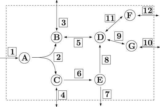
Example of a metabolic network. The set of internal metabolites is $\mathfrak{M}=\{A,B,\dots ,G\}$⁠. The set of reactions is $\mathfrak{R}=\{1,2,\dots ,11,12\}$⁠, where the irreversible reactions are $\text{Irr}=\{1,2,6,7,8\}$⁠. The stoichiometric coefficients $S_{i,j}$ are assumed to be in $\{-1,0,1\}$⁠. If reaction 7 is the target reaction we have the following MCSs: If reaction 6 is not present, e.g. knocked out, there is no flux through reaction 7. Therefore reaction 6 is an MCS of cardinality 1. If the reactions 2 and 4 are not present, there is no flux through reaction 7. Therefore reactions 2 and 4 form an MCS of cardinality 2

This work is about subsets of reactions $\zeta \subset \mathfrak{R}$ that are called cut sets. If the reactions in ζ are removed from $\mathcal{N}$⁠, other reactions called target reactions are not able to carry non-zero flux anymore. A cut set ζ is called (inclusion-)minimal if no proper subset of ζ is a cut set for the pre-defined target reactions. Minimal cut sets (MCSs) were first introduced in Klamt and Gilles (2004) and have many applications (Apaolaza et al., 2017; Clark and Verwoerd, 2012; Gerstl et al., 2016; Gruchattka et al., 2013; Harder et al., 2016; Imielinski and Belta, 2008; Klamt, 2006; Machado and Herrgård, 2015; von Kamp and Klamt, 2017; Wilhelm et al., 2004). Various methods exist to compute MCSs (Ballerstein et al., 2012; Goldstein and Bockmayr, 2015; Haus et al., 2008; Jungreuthmayer et al., 2013; Nair et al., 2017; Tobalina et al., 2016; von Kamp and Klamt, 2014).

One of the very first methods to compute MCSs (Klamt, 2006; Klamt and Gilles, 2004) is to use the set of all elementary flux modes (EFMs). EFMs (Schuster and Hilgetag, 1994) are flux vectors $v\in {\Gamma }_{\mathcal{N}}$ with (inclusion-)minimal support, where the support $\mathrm{supp}(v):=\left\{i\in \mathfrak{R}|v_i\cancel{=}0\right\}$ is the set of active reactions in v. One can show that, up to scaling, an EFM is uniquely determined by its support. Therefore, two EFMs $e,e\prime$ are considered to be the same if $\mathrm{supp}(e)=\mathrm{supp}(e\prime )$⁠. The set of all EFMs defines a generating set for the flux cone ${\Gamma }_{\mathcal{N}}$⁠. This means that every flux vector $v\in {\Gamma }_{\mathcal{N}}$ can be represented as a conical combination $v=\sum _{e\in \text{EFMs}}{\lambda }_{e}e$ with ${\lambda }_e\ge 0$⁠. Thus, every (steady-state) behaviour of the network can be represented with the help of EFMs. Over the last 20 years, various methods have been developed to compute the set of all EFMs in a given metabolic network (Fukuda and Prodon, 1996; Gagneur and Klamt, 2004; Pfeiffer et al., 1999; Terzer, 2009; Urbanczik and Wagner, 2005b).

The procedure to compute MCSs using EFMs (Klamt, 2006) works as follows: Suppose all EFMs are known and a target reaction is given. Let ${\text{EFMs}}_{\text{tar}}$ be the set of those EFMs that involve the target reaction. Given ${\text{EFMs}}_{\text{tar}}$⁠, we search for hitting sets, i.e. sets of reactions such that each EFM in ${\text{EFMs}}_{\text{tar}}$ contains at least one reaction of the hitting set. Inclusion-minimal hitting sets are the MCSs we are looking for.

 

Example 1

(Using EFMs to compute MCSs) For the network in Figure 1 there exist 18 EFMs, a complete list can be found in Supplementary Material, Section 1. We choose reaction 7 as the target reaction. There are four EFMs using reaction 7 with the supports $\{1,2,3,6,7\},\hspace{0.17em}\{1,2,5,6,7,9,10\},\hspace{0.17em}\{1,2,5,6,7,11,12\}$⁠, {4, 6, 7}. In all these EFMs, reaction 6 is active. Therefore, if reaction 6 is removed, there will be no feasible flux vector using reaction 7. Consequently, the set {6} is an MCS for the target reaction 7. MCSs of cardinality 2 are {1, 4} and {2, 4}. The set {1, 6} is not an MCS since it contains the MCS {6}. The remaining MCSs are $\{3,4,5\},\{3,4,9,11\},\{3,4,10,12\},\{3,4,10,11\},\{3,4,9,12\}$⁠.

A second way to compute MCSs is based on the Farkas’ lemma and linear programming duality (Ballerstein et al., 2012; Larhlimi and Bockmayr, 2007; von Kamp and Klamt, 2014). As shown in Ballerstein et al. (2012), the MCSs in a network $\mathcal{N}$ for a given target reaction $t\in \mathfrak{R}$ correspond to EFMs in a dual network${\mathcal{N}}_t^{*}$⁠. Intuitively speaking, the metabolites in ${\mathcal{N}}_t^{*}$ correspond to the reactions in $\mathcal{N}$ and vice versa. The stoichiometric matrix of ${\mathcal{N}}_t^{*}$ is the transposed stoichiometric matrix of the primal network $\mathcal{N}$⁠, where some columns have to be added. Exploiting this duality, one can use mixed integer linear programming (MILP) to enumerate MCSs of increasing size (Larhlimi and Bockmayr, 2007; von Kamp and Klamt, 2014). Further extending these methods, Tobalina et al. (2016) compute MCSs that contain a pre-defined knock-out reaction $t\prime \ne t$ by enumerating EFMs in the dual network ${\mathcal{N}}_t^{*}$ in which $t\prime$ is active.

Computing MCSs via EFMs, either in the primal or in the dual network, gets the more and more difficult, the larger these networks become. To address this problem, we propose here to use projections in order to reduce the size of the underlying polyhedral cones. The projection of the flux cone ${\Gamma }_{\mathcal{N}}$ onto the set of irreversible reactions $\text{Irr}$ leads to a smaller cone ${\mathrm{proj}}_{\text{Irr}}({\Gamma }_{\mathcal{N}})$⁠, which is again a flux cone, but where only irreversible reactions are active. To compute MCSs, we can apply the methods explained before to ${\mathrm{proj}}_{\text{Irr}}({\Gamma }_{\mathcal{N}})$ instead of ${\Gamma }_{\mathcal{N}}$ in order to compute MCSs. The resulting cuts are MCSs of $\mathcal{N}$ that consist of irreversible reactions only. Therefore, we call them irreversible minimal cut sets (iMCSs).

 

Definition 1

(iMCSs) Given a metabolic network $\mathcal{N}=(\mathfrak{M},\mathfrak{R},S,\text{Irr})$ a set of reactions $\zeta \subset \mathfrak{R}$ is called a cut set for a target reaction $t\in \mathfrak{R}$⁠, if v_t = 0 for all flux vectors $v\in {\Gamma }_{\mathcal{N}}$ with v_i = 0, for all $i\in \zeta$⁠. For $t\in \mathfrak{R}$⁠, an iMCS is an (inclusion-)MCSs $\zeta \subset \text{Irr}$ consisting of irreversible reactions only.

We will show that the EFMs of the projection ${\mathrm{proj}}_{\text{Irr}}({\Gamma }_{\mathcal{N}})$ are the minimal metabolic behaviours (MMBs) of the network $\mathcal{N}$⁠. A metabolic behaviour (Larhlimi and Bockmayr, 2009) is a non-empty set of irreversible reactions $D\subseteq \text{Irr}$ that are active together in some flux vector $v\in {\Gamma }_{\mathcal{N}}$⁠, i.e. $D=\{i\in \text{Irr}|v_i\cancel{=}0\}$⁠. A metabolic behaviour is minimal if there is no metabolic behaviour $D\prime$ strictly contained in D. This definition is similar to the one of EFMs with the difference that in the case of MMBs only irreversible reactions are considered. The number of MMBs may be by several orders of magnitude smaller than the number of EFMs, see Larhlimi and Bockmayr (2009) and Table 1. We can use MMBs in the same way as EFMs in order to compute iMCSs instead of MCSs. Suppose the whole set of MMBs is known and an irreversible target is chosen. The set ${\text{MMBs}}_{\text{tar}}$ consists of all MMBs which contain the target reaction. Within ${\text{MMBs}}_{\text{tar}}$ minimal hitting sets are searched, which are MCSs. Since they consist of irreversible reactions only, they are iMCSs, see Example 2 for illustration.

Table 1.

Comparison of the number of EFMs, number of MMBs, number of target MMBs, number of iMCSs and time to compute these sets for different networks

Network	rxns	irr	MMBs	EFMs	Time MMBs (s)	Target MMBs	iMCSs	Time iMCSs
Escherichia coli MG1655 (Orth et al., 2010)	87	41	2572	100 274	5.7	1151	257	113 s
Rhizobium etli iOR363 (Resendis-Antonio et al., 2007)	194	104	6147	N/A	26	651	60	60 s
Buchnera iSM197 (MacDonald et al., 2011)	244	170	245	N/A	7	146	200	130 s
Blattabacterium cuenoti iCG238 (González-Domenech et al., 2012)	308	197	374	N/A	7.7	128	184	138 s
Blattabacterium iCG230 (González-Domenech et al., 2012)	400	192	82	N/A	6.7	32	159	115 s
Mycobacterium tuberculosis iNJ661 (Jamshidi and Palsson, 2007)	427	296	501	N/A	13	350	381	449 s
Salmonella Typhimurium STM_v1_0 (Thiele et al., 2011)	458	316	97	N/A	11.8	96	321	386 s
Helicobacter pylori iCS291 (Schilling et al., 2002)	444	271	150, 132	N/A	325	148 608	187	5 h 44 min 1 s

Note: Network: name of the metabolic network. rxns: number of unblocked reactions of the network. irr: number of unblocked irreversible reactions of the network. MMBs: number of MMBs. EFMs: number of EFMs. N/A: the programmes used here (polco and efmtool, http://www.csb.ethz.ch/tools/software) could not handle the size of the models resp. the number of EFMs. Time MMBs: Time to compute MMBs using projection. Target MMBs: number of MMBs involving the target reaction (biomass reaction). iMCS: number of iMCSs. Time iMCSs: time to compute iMCSs. The description of E.coli MG1655 (Orth et al., 2010) was taken from the BiGG Models Database (King et al., 2016), while the remaining ones are all taken from BioModels Database (Li et al., 2010).

 

Example 2

(Using MMBs to compute iMCSs) The network in Figure 1 has three different MMBs: $\{1,2\},\{6,7\}$ and {6, 8}. We apply the method from Example 1 to compute MCSs, but instead of EFMs we now use MMBs. The target reaction is again reaction 7. The only MMB containing reaction 7 is {6, 7}. Therefore, the iMCSs for reaction 7 are {6} and {7}.

Using MMBs instead of EFMs will allow us to compute (irreversible) MCSs for larger networks, see Section 4. However, there are still limits. In practice, it is often not possible to compute the MMBs for genome-scale metabolic networks. Nevertheless, we can still perform the projection and then apply MILP techniques on the dual projected cone ${\mathrm{proj}}_{\text{Irr}}{({\Gamma }_{\mathcal{N}})}_t^{*}$⁠, using the method of von Kamp and Klamt (2014) or Tobalina et al. (2016). The classical method to perform projections is Fourier–Motzkin elimination, see e.g. (Ziegler, 1995). In general, Fourier–Motzkin elimination leads to a combinatorial explosion in the number of linear inequalities needed to describe the projected cone. However, in the special case of flux cones, we can use the theory of oriented matroids to avoid this if we project along reversible reactions on the set of irreversible reactions. This enables us to perform the projection efficiently also on genome-scale metabolic networks.

To summarize, the contributions of this paper are the following:

• We introduce the new concept of iMCSs.

• We present an efficient method to project a metabolic network onto its irreversible reactions, based on contraction of oriented matroids.

• We present a new method for computing MMBs and two approaches for computing iMCSs.

• We illustrate our theoretical results by various computational experiments.

2 Mathematical background

We start by providing some mathematical background needed to develop our method. For a vector $x\in {\mathbb{R}}^n$ and a set of indices $I\subseteq \{1,\dots ,n\}$ we denote by x_I the subvector consisting of the components x_i with $i\in I$⁠. We use superscripts to refer to several vectors such as $x^1,\dots ,x^s$⁠. For a matrix $A\in {\mathbb{R}}^{m\times n}$ we denote by $A_{I,*}$ resp. $A_{*,I}$ the submatrix consisting of the rows resp. columns whose indices belong to I. The rank or maximum number of linearly independent columns in A is denoted by $\rho (A)$⁠. The identity matrix is denoted by $E\in {\mathbb{R}}^{n\times n}$⁠.

Next we give some basic definitions and theorems related to polyhedral cones, see Schrijver (1998) for more details. A subset $\Gamma \subseteq {\mathbb{R}}^n$ is called a cone if any conic combination of two elements $x,y\in \Gamma$ belongs to Γ again, i.e. $\lambda x+\mu y\in \Gamma$⁠, for any non-negative $\lambda ,\mu \in {\mathbb{R}}_{\ge 0}$⁠. A cone Γ is called polyhedral if there exists a matrix $A\in {\mathbb{R}}^{m\times n}$ such that $\Gamma =\left\{x\in {\mathbb{R}}^n|Ax\ge 0\right\}$⁠. A cone Γ is finitely generated if there exists a finite set of generators $\{g^1,\dots ,g^s\}\subseteq \Gamma$ such that every element $x\in \Gamma$ can be written in the form $x={\sum }_{k=1}^s{\lambda }_k{g}^k$⁠, for some non-negative ${\lambda }_k\in {\mathbb{R}}_{\ge 0}$⁠. By a classical theorem of Farkas–Minkowski–Weyl, a cone is polyhedral if and only if it is finitely generated. For a polyhedral cone Γ, the linear subspace $\Lambda =\left\{x\in {\mathbb{R}}^n|Ax=0\right\}$ is called the lineality space of Γ. The cone Γ is called pointed if $\Lambda =\left\{0\right\}$⁠. This means that whenever $x\in \Gamma \setminus \left\{0\right\}$⁠, we have $-x\cancel{\in }\Gamma$⁠. In other words, Γ does not contain any line $\{\lambda x|\lambda \in \mathbb{R}\}$⁠, for $x\ne 0$⁠. By basic linear algebra, a cone Γ is pointed if and only if the matrix A has full column rank, i.e. $\rho (A)=n$⁠. A ray is a non-zero element of Γ and two rays $x,x\prime$ are considered identical if $x\prime =\lambda x$ for some $\lambda >0$⁠. A ray x is called an extreme ray of Γ, if there exist no two linearly independent rays $x^1,x^2\in \Gamma$ such that $x=x^1+x^2$⁠. If Γ is pointed, the extreme rays form a unique minimum set of generators $\{g^1,\dots ,g^s\}\subseteq \Gamma$⁠, see Figure 2 for illustration.

Fig. 2.

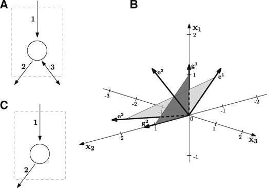
(A) Metabolic network $\mathcal{N}$ involving three reactions, where the third one is reversible. The network has three EFMs: $e^1=(1,0,1),\hspace{0.17em}{e}^2=(0,1,-1)$ and $e^3=(1,1,0)$⁠. (B) The corresponding flux cone $\Gamma =\{x\in {\mathbb{R}}^3|x_1-x_2-x_3=0,x_1,x_2\ge 0\}$⁠, shown in light grey, is a pointed cone and spanned by the EFMs e¹ and e², which are the extreme rays of the cone. The third EFM e³ lies inside Γ and is a conic combination of e¹ and e². The lineality space is {0}. Projecting Γ in direction of the reversible reaction 3 results in the projected cone ${\mathrm{proj}}_{\{1,2\}}(\Gamma )=\{x\in {\mathbb{R}}^3|x_3=0,x_1,x_2\ge 0\}$⁠, shown in dark grey. It is again a pointed cone and is generated by the vectors $g^1=(1,0,0)$ and $g^2=(0,1,0)$⁠, which correspond to the two MMBs {1} and {2} of $\mathcal{N}$⁠. (C) Removing reaction 3 results in the network in (C), which has only one EFM, namely e¹

In the following, we consider a special class of polyhedral cones, which we call flux cones:

 

Definition 2

(Flux cone) A polyhedral cone Γ is called a flux cone if there exists a matrix $B\in {\mathbb{R}}^{m\times n}$ and an index set $I\subseteq \{1,\dots ,n\}$ such that

$$\Gamma =\{x\in {\mathbb{R}}^n|\left(\begin{array}{c}B\\ -B\\ E_{I,*}\end{array}\right)x\ge 0\}=\{x\in {\mathbb{R}}^n|Bx=0,\hspace{0.17em}{x}_I\ge 0\}.$$

Either B or I may be empty, but not both.

Clearly, the flux cone ${\Gamma }_{\mathcal{N}}$ of a metabolic network $\mathcal{N}=(\mathfrak{M},\mathfrak{R},S,\text{Irr})$ is a flux cone in the sense of Definition 2, with B = S and $I=\text{Irr}$⁠.

 

Proposition 1

Let Γ be a flux cone. If $x\ge 0$ for all $x\in \Gamma$⁠, then Γ is pointed and the extreme rays of Γ are exactly the rays in Γ of minimal support.

The proof of Proposition 1 and all the following proofs can be found in Supplementary Material, Section 5.

In general, metabolic networks may contain reversible reactions together with reversible flux vectors $v\ne 0$ for which $v,-v\in {\Gamma }_{\mathcal{N}}$⁠. For example in Figure 1, there is a reversible flux vector with support $\{3,5,9,10\}$⁠. In such networks, the flux cone is not pointed, and Proposition 1 does not apply. If there exist reversible reactions but the flux cone is still pointed, then all extreme rays have minimal support, but the converse is no longer true.

3 Materials and methods

As explained in the Section 1, our goal is to compute (irreversible) MCSs for genome-scale networks $\mathcal{N}$ by computing MCSs of the projected cone ${\mathrm{proj}}_{\text{Irr}}({\Gamma }_{\mathcal{N}})$⁠. Since ${\mathrm{proj}}_{\text{Irr}}({\Gamma }_{\mathcal{N}})$ is usually smaller than ${\Gamma }_{\mathcal{N}}$⁠, this will allow us to handle larger metabolic networks and to compute (irreversible) MCSs more efficiently.

3.1 Projection of flux cones

Projections of the flux cone of a metabolic network have been considered before in the literature (Covert and Palsson, 2003; Marashi et al., 2012; Urbanczik, 2006; Urbanczik and Wagner, 2005a; Wagner and Urbanczik, 2005; Wiback and Palsson, 2002). For $x\in {\mathbb{R}}^n$ and $H\subseteq \{1,\dots ,n\}$ the projection of x on H is defined as ${\mathrm{proj}}_H(x)=(x_H,0)$⁠. Similarly, for a polyhedral cone $\Gamma \subseteq {\mathbb{R}}^n$⁠, let ${\mathrm{proj}}_H(\Gamma )=\{{\mathrm{proj}}_H(x)|x\in \Gamma \}$⁠. It is well known that ${\mathrm{proj}}_H(\Gamma )$ is again a polyhedral cone (Ziegler, 1995).

Here we show that the projection ${\mathrm{proj}}_H({\Gamma }_{\mathcal{N}})$ of the flux cone ${\Gamma }_{\mathcal{N}}$ of a metabolic network $\mathcal{N}=(\mathfrak{M},\mathfrak{R},S,\text{Irr})$ will be again a flux cone in the sense of Definition 2, if we project along one or more reversible reactions on a superset $H\supseteq \text{Irr}$ of the set of irreversible reactions.

 

Theorem 1

Let  $\Gamma =\{x\in {\mathbb{R}}^n|Ax\ge 0\}$ be a flux cone with $A=\left(\begin{array}{c}B\\ -B\\ E_{I,*}\end{array}\right)$. For any$H\supseteq I$ the projection ${\mathrm{proj}}_H(\Gamma )$ is again a flux cone.

In the following, we consider the special case of flux cones $\Gamma ={\Gamma }_{\mathcal{N}}$ and $H=\text{Irr}$⁠. This means that we project along all the reversible reactions on the set of all irreversible reactions. By Theorem 1, the projection ${\mathrm{proj}}_{\text{Irr}}({\Gamma }_{\mathcal{N}})$ is again a flux cone in the sense of Definition 2. Every vector $(v_{\text{Irr}},0)\in {\mathrm{proj}}_{\text{Irr}}({\Gamma }_{\mathcal{N}})$ can be lifted to a vector $v=(v_{\text{Irr}},v_{\text{Rev}})\in {\Gamma }_{\mathcal{N}}$ of the original network by adding suitable components for the reversible reactions. The flux cone ${\mathrm{proj}}_{\text{Irr}}({\Gamma }_{\mathcal{N}})$ is pointed since only irreversible reactions can be active. However, ${\mathrm{proj}}_{\text{Irr}}({\Gamma }_{\mathcal{N}})$ does not necessarily describe a metabolic network. An example is given in Figure 2, which shows that projecting the flux cone along a reversible reaction is different from deleting this reaction from the network.

3.2 Computing MMBs via projection

We next show that the MMBs of a metabolic network $\mathcal{N}$ can be obtained from the extreme rays of the pointed cone ${\mathrm{proj}}_{\text{Irr}}({\Gamma }_{\mathcal{N}})$⁠.

 

Theorem 2

Let ${\Gamma }_{\mathcal{N}}=\{v\in {\mathbb{R}}^{\left|\mathfrak{R}\right|}|Sv=0,\hspace{0.17em}{v}_{\text{Irr}}\ge 0\}$ be the flux cone of a metabolic network $\mathcal{N}=(\mathfrak{M},\mathfrak{R},S,\text{Irr})$⁠. The supports of the extreme rays of the pointed cone ${\mathrm{proj}}_{\text{Irr}}({\Gamma }_{\mathcal{N}})$ are exactly the MMBs of the network $\mathcal{N}$⁠.

Up to now there are three ways for enumerating all MMBs in a metabolic network. The first one is to compute all EFMs and to search for the MMBs contained in them. Since this method involves enumerating the whole set of EFMs, it is usually not applicable to genome-scale networks. A closely related approach is to compute a minimum set of generators for the flux cone, e.g. by using the double description method (Fukuda and Prodon, 1996). The supports of the generators that do not belong to the lineality space then correspond to the MMBs (Larhlimi and Bockmayr, 2009). A third method is using MILP (Rezola et al., 2011) to compute so-called generating flux modes, from which again the MMBs can be obtained.

Theorem 2 leads to a new approach for computing the set of MMBs of a metabolic network $\mathcal{N}$⁠. First compute an inequality description of the projection ${\mathrm{proj}}_{\text{Irr}}({\Gamma }_{\mathcal{N}})$⁠, then compute the extreme rays of ${\mathrm{proj}}_{\text{Irr}}({\Gamma }_{\mathcal{N}})$ and their supports.

3.3 Projection and contraction

In this section, we apply the theory of oriented matroids to give an efficient procedure for computing an inequality description of the cone ${\mathrm{proj}}_{\text{Irr}}({\Gamma }_{\mathcal{N}})$⁠. The classical method for projection of polyhedral cones is Fourier–Motzkin elimination (Ziegler, 1995). In general, this can lead to a combinatorial explosion in the number of linear inequalities needed to describe the projected cone. In our case we are concerned with the special case of flux cones of the form $\Gamma =\{x\in {\mathbb{R}}^n|Ax\ge 0\}$ with $A=\left(\begin{array}{c}B\\ -B\\ E_{I,*}\end{array}\right)$⁠, and we always project along components $k\cancel{\in }I$⁠. As we will see, this implies that all changes in the row structure of A during projection will occur in the equational part Bx = 0, while the matrix $E_{I,*}$ representing the linear inequalities is not changed (cf. the proof of Theorem 1 in Supplementary Material, Section 5). Since the homogeneous linear equation system Bx = 0 describes an oriented matroid (Björner et al., 1999), the projection of flux cones can be performed efficiently via contraction of oriented matroids.

Let U be a set. A signed subset of U is a pair $X=(X^{+},X^{-})$ with a set of positive elements $X^{+}\subseteq U$ and a set of negative elements $X^{-}\subseteq U$ such that $X^{+}\cap X^{-}=\varnothing$⁠. The support of X is the set $\mathrm{supp}(X)=X^{+}\cup X^{-}$⁠. An oriented matroid is a pair $\mathcal{M}=(U,\mathcal{C})$⁠. Here U is a set and $\mathcal{C}$ is a family of signed subsets of U, called the oriented circuits of $\mathcal{M}$⁠, which satisfy the circuit axioms that can be found in Supplementary Material, Section 2, or Björner et al. (1999). The equivalent of projection for oriented matroids is called contraction. Let $\mathcal{M}=(U,\mathcal{C})$ be an oriented matroid. For $X\in \mathcal{C}$ and $H\subseteq U$ we denote by $X{|}_H$ the signed set $(X^{+}\cap H,X^{-}\cap H)$⁠. The family $\text{Min}(\{X{|}_H|X\in \mathcal{C}\})$ of non-empty intersections of circuits of $\mathcal{M}$ with H that have inclusion-minimal support is the set of circuits of an oriented matroid on H (Björner et al., 1999). This matroid is called the contraction of$\mathcal{M}$to H and will be denoted by ${\text{contr}}_H(\mathcal{M})$⁠.

In our case, we consider a special class of matroids which are called representable. Let $B\in {\mathbb{R}}^{m\times \left|U\right|}$ be a matrix and let U be the set of columns of B. The oriented matroid${\mathcal{M}}_B=(U,\mathcal{C})$represented by B is given by $\mathcal{C}=\mathrm{Min}(\mathcal{V})$⁠, where $\mathcal{V}=\{\sigma (x)|Bx=0,\hspace{0.17em}x\in {\mathbb{R}}^{\left|U\right|}\}$⁠. Here $\sigma (x)$ denotes the signed set obtained by applying the sign function component-wise to the vector x, and $\mathrm{Min}(\mathcal{V})$ is the set of non-empty signed sets in $\mathcal{V}$ with inclusion-minimal support. The matrix representing the contraction ${\text{contr}}_H({\mathcal{M}}_B)$ of the oriented matroid ${\mathcal{M}}_B$ can be computed by basic linear algebra, see Supplementary Material, Section 3. There is no combinatorial explosion like in Fourier–Motzkin elimination.

 

Theorem 3

The MMBs of a metabolic network $\mathcal{N}=(\mathfrak{M},\mathfrak{R},S,\text{Irr})$ with flux cone ${\Gamma }_{\mathcal{N}}$ are exactly the oriented circuits X of the contraction ${\text{contr}}_{\text{Irr}}({\mathcal{M}}_S)$ for which $X^{-}=\varnothing$⁠. If $T\in {\mathbb{R}}^{k\times \left|\text{Irr}\right|}$ is a matrix representing ${\text{contr}}_{\text{Irr}}({\mathcal{M}}_S)$ then

$${\mathrm{proj}}_{\text{Irr}}({\Gamma }_{\mathcal{N}})=\{v\in {\mathbb{R}}^{\left|\mathfrak{R}\right|}|T{v}_{\text{Irr}}=0,v_{\text{Irr}}\ge 0,v_{\text{Rev}}=0\}.$$

 

Example 3

Consider again the network $\mathcal{N}=(\mathfrak{M},\mathfrak{R},S,\text{Irr})$ in Figure 1. Let ${\mathcal{M}}_S=(\mathfrak{R},\mathcal{C})$ be the oriented matroid represented by the stoichiometric matrix $S\in {\mathbb{R}}^{\left|\mathfrak{M}\right|\times \left|\mathfrak{R}\right|}$⁠. This matroid contains 24 oriented circuits, where we identify two oriented circuits X and Y if $X=-Y$⁠. Among those, 18 correspond to EFMs, e.g. $\{+1,+2,+3,+4\}$ or $\{-4,+6,+7\}$⁠. The remaining six oriented circuits $\{-7,+8,+9,+10\},\{+1,+2,+4,+5,+7,-8\},\{-3,+5,+7,-8\},\{+1,+2,+5,+6,+7,-8\},\{+1,+2,+4,+5,-6,-8\},\{-7,+8,+11,+12\}$ do not correspond to a feasible flux vector. In each of these, there is an irreversible reaction with negative flux. Contracting ${\mathcal{M}}_S$ on $\text{Irr}$ results in the oriented matroid ${\text{contr}}_{\text{Irr}}({\mathcal{M}}_S)$ represented by the matrix

$$\begin{array}{c}\hspace{0.17em}\hspace{0.17em}\hspace{0.17em}\hspace{0.17em}\hspace{0.17em}\hspace{0.17em}\hspace{0.17em}\hspace{0.17em}\hspace{0.17em}\hspace{0.17em}\hspace{0.17em}\hspace{0.17em}\hspace{0.17em}\hspace{0.17em}\hspace{0.17em}\hspace{0.17em}\hspace{0.17em}\begin{array}{ccccc}1\hfill & \hspace{0.17em}\hspace{0.17em}\hspace{0.17em}2\hfill & 6\hfill & 7\hfill & \hspace{0.17em}\hspace{0.17em}\hspace{0.17em}8\hfill \end{array}\\ T=\begin{array}{c}A\\ E\end{array}\left(\begin{array}{ccccc}1\hfill & -1\hfill & 0\hfill & 0\hfill & 0\hfill \\ 0\hfill & 0\hfill & 1\hfill & -1\hfill & -1\hfill \end{array}\right),\end{array}$$

for the details, see Supplementary Material, Section 3, Example 1.

By Theorem 3, the matrix T also describes the flux cone ${\mathrm{proj}}_{\text{Irr}}({\Gamma }_{\mathcal{N}})=\{v\in {\mathbb{R}}^{\left|\mathfrak{R}\right|}|T{v}_{\text{Irr}}=0,\hspace{0.17em}{v}_{\text{Irr}}\ge 0,\hspace{0.17em}{v}_{\text{Rev}}=0\}$⁠, in which all active reactions are irreversible. By Proposition 1, the extreme rays of ${\mathrm{proj}}_{\text{Irr}}({\Gamma }_{\mathcal{N}})$ are exactly the EFMs of the network represented by ${\mathrm{proj}}_{\text{Irr}}({\Gamma }_{\mathcal{N}})$⁠, which is shown in Figure 3. The supports of these extreme rays are $\{1,2\},\{6,7\},\{6,8\}$⁠, which are the MMBs of the original network from Figure 1. The oriented circuits of ${\text{contr}}_{\text{Irr}}({\mathcal{M}}_S)$ include these MMBs (as signed sets) and one additional oriented circuit $\{-7,+8\}$⁠.

Fig. 3.

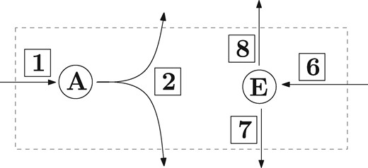
Projection of the network in Figure 1 on the set of irreversible reactions. Reactions 1 and 2 are independent from reactions 6, 7 and 8. The metabolites that were connected to the reversible reactions have been removed

4 Results and discussion

To illustrate our method, we describe a number of computational experiments for computing (irreversible) MCSs based on the projection of the flux cone. For lack of space, we highlight here only some of the results using overview figures. Full tables with all the data can be found in Supplementary Material, Section 6. All computations were done on a desktop computer with eight processors Intel(R) Core(TM) i7-2600, CPU 3.40 GHZ, each with two threads. When searching for MCSs in the original flux cone, we only allowed irreversible reactions to be included in the computed MCSs. Thus, we computed iMCSs as well, but without performing the projection.

4.1 Computing iMCSs using MMBs

We first consider the hitting set approach. Instead of EFMs we use MMBs, which correspond to the extreme rays (or EFMs) of ${\mathrm{proj}}_{\text{Irr}}({\Gamma }_{\mathcal{N}})$ (cf. Theorem 2). It is known that the number of MMBs is typically much smaller than the number of EFMs (Larhlimi and Bockmayr, 2009). For computing the MMBs, we implemented the approach from Section 3.2 in MATLAB. We used the software SAGE (http://www.sagemath.org) (The Sage Developers, 2016) for computing the projection via contraction and the software polco (Terzer, 2009) for enumerating the extreme rays. Given the set of MMBs, computing iMCSs becomes a hitting set problem, see Supplementary Material Section 4 or Klamt (2006).

To evaluate our method, we considered a selection of medium-sized metabolic networks from the BioModels Database (Li et al., 2010). The number of unblocked reactions, i.e. reactions whose steady-state flux is not always zero, ranges from 87 up to 444. While EFMs could be computed for only one network, the set of MMBs could be obtained for all these networks in a relatively short amount of time, see Table 1.

All these networks contain a biomass reaction, which we used as target reaction for computing the iMCSs. The hitting set approach allowed us to enumerate all iMCSs for these networks, see Supplementary Table S3. For several networks, the maximal cardinality of the iMCSs did not exceed 5 and most iMCSs have even cardinality 1. In Blattabacterium iCG230, we only have iMCSs of cardinality 1 (152 iMCSs) and cardinality 2 (7 iMCSs). Salmonella Typhimurium STM_v1_0 is another example with 296 iMCSs of cardinality 1, 19 of cardinality 2 and 6 of cardinality 3.

4.2 Computing iMCSs using the dual approach

The network sizes for which we are able to compute the MMBs are still limited. The bottleneck is computing the extreme rays of ${\mathrm{proj}}_{\text{Irr}}({\Gamma }_{\mathcal{N}})$ by polco (Terzer, 2009), while doing the projection is feasible even for very large networks. We performed the projection on the set of irreversible reactions for all 84 networks of the BiGG Models Database (King et al., 2016), using SAGE (The Sage Developers, 2016) for the contraction. This took between 32 s (for a network of 87 unblocked reactions) and 35 min (for a network of 4047 unblocked reactions), see Figure 1 and Supplementary Tables S1 and S2.

Next we used the resulting matrices describing ${\mathrm{proj}}_{\text{Irr}}({\Gamma }_{\mathcal{N}})$ for computing k-shortest iMCSs by the method of von Kamp and Klamt (2014), which is part of CellNetAnalyzer version 2018.1 (von Kamp et al., 2017). As MILP solver, we used CPLEX 12.8 (http://www.cplex.com). Compared to using the full flux cone, we were able to compute more iMCSs and in shorter time, see Figure 4 and Supplementary Tables S4–S7. Note that for various larger genome-scale metabolic networks, it was not possible to compute any iMCSs using the original cone, while in all these cases we were able to compute 40 or more iMCSs using the projected cone (see Supplementary Tables S6 and S7). In general, we can observe that the benefits from using the projection increase with the size of the network.

Fig. 4.

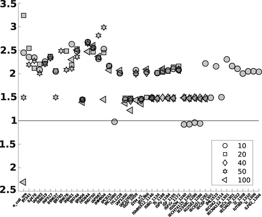
We consider here all networks from the BiGG Models Database where we were able to compute iMCSs both in the original and in the projected flux cone. The ids of the networks can be found on the x-axis. The networks are ordered by the number of reactions. For each number of iMCSs to be computed (10, 20, 40, 50 or 100) there exists a differently shaped marker. Its position indicates the relative time (y-axis) needed to compute the given number of iMCSs in the original versus the projected flux cone. If the marker is above the line, this means that using the projected cone is faster. As one can see, computing 20, 40 or 50 iMCSs is always faster with the projected cone. For example, computing 50 iMCSs for the network iAF692 is roughly two times faster in the projected cone. If the marker is below the line, it is faster to use the original cone. For example, computing 100 iMCSs for the network e_coli_core is roughly 2.4 times faster in the original cone. Altogether, the figure shows that in most instances, it is faster to use the projected cone. For details, we refer to Supplementary Tables S4–S7

Finally we considered the computation of iMCSs containing a specific reaction knock-out. We applied the software of Tobalina et al. (2016) together with CPLEX 12.4 to the original stoichiometric matrices as well as to the reduced matrices after projection, and compared the results. Like in Tobalina et al. (2016), we used the biomass as target reaction. For each irreversible reaction, we set a time limit of 1 min to compute a single iMCS that contains this reaction. If no iMCS could be found within 1 min, the computation was stopped and we moved on to the next irreversible reaction. We report on the 39 networks in the BiGG database for which the total computation time for this experiment did not exceed 3 days. Except for one network, we were able to compute more iMCSs using the projection, see Figure 5 and Supplementary Table S8.

Fig. 5.

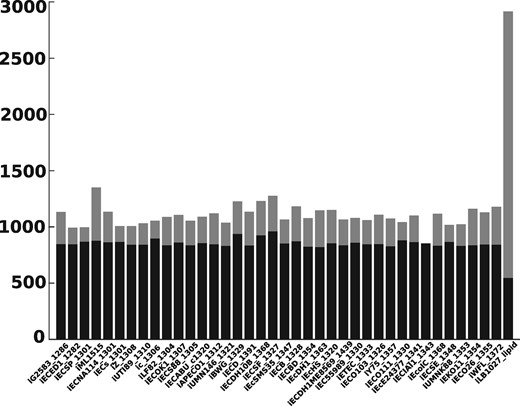
We consider here all networks from the BiGG Models Database for which the total computation time for the method of Tobalina et al. (2016) took <3 days. The biomass reaction is the target reaction for computing iMCSs and one additional irreversible reaction is defined as a knock-out reaction. We loop over all irreversible reactions. In step i, reaction i is defined as the knock-out reaction and we try to compute an iMCS for the target reaction containing i. After 1 min or if an iMCS has been found, the next step starts. The y-axis indicates the number of iMCSs that were found. The transparent bar (which includes the non-transparent bar) indicates the number of iMCSs computed using the projected cone. The non-transparent bar indicates the number of iMCSs computed for the original cone. Except for one network, we were able to compute more iMCSs using the projected cone. For details, see Supplementary Table S8

5 Conclusion

We introduced the new concept of iMCSs and presented different ways for computing them. On the algorithmic side, the key idea is the projection of flux cones, which is done by the contraction of an oriented matroid. Our first approach to compute iMCSs uses MMBs. To find the MMBs of a metabolic network $\mathcal{N}$⁠, we project the flux cone ${\Gamma }_{\mathcal{N}}$ on the set of irreversible reactions $\text{Irr}$⁠. The supports of the extreme rays of the pointed cone ${\mathrm{proj}}_{\text{Irr}}({\Gamma }_{\mathcal{N}})$ are the MMBs of $\mathcal{N}$⁠.

A second way for computing iMCSs consists in applying to the projected cone ${\mathrm{proj}}_{\text{Irr}}({\Gamma }_{\mathcal{N}})$ the dual approach for computing (irreversible) MCSs (Tobalina et al., 2016; von Kamp and Klamt, 2014). Using the projection we are able to compute iMCSs in most cases faster and in networks where the standard method (using the original cone) fails, due to lack of memory. Since we can only compute irreversible MCSs with our approach, it may happen that certain MCSs of interest are missed, e.g. MCSs which are easy to implement in the wet lab. If no irreversible MCSs exist or if certain reversible reactions are of particular importance, the projection can be performed on those reversible reactions, too. The only restriction is that all irreversible reactions have to preserve in the projected cone. A possible direction for future research is computing constrained iMCSs (Hädicke and Klamt, 2011) or applying other constraint-based methods to the projected cone ${\mathrm{proj}}_{\text{Irr}}({\Gamma }_{\mathcal{N}})$⁠.

While large MCSs are hard to use for wet lab experiments, they allow studying the fragility of a metabolic network (Clark and Verwoerd, 2012; Gerstl et al., 2016; Klamt, 2006; Klamt and Gilles, 2004). Since the fragility of a network (resp. of a pre-defined reaction $i\in \mathfrak{R}$⁠) is given by the size distribution over the total set of MCSs (resp. the set of MCSs including i), all MCSs have to be known. For example, Klamt and Gilles (2004) found MCSs indicating that in the central metabolism of Escherichia coli growth on glucose is less fragile (more robust) than growth on acetate. While iMCSs do not cover the whole set of MCSs, they give the possibility to compute MCSs of larger cardinality, which may give additional biological insights.

Acknowledgement

We thank Alexandra M. Reimers for fruitful discussions and comments on this work.

Conflict of Interest: none declared.