Boost-HiC: computational enhancement of long-range contacts in chromosomal contact maps

Abstract

Motivation

Genome-wide chromosomal contact maps are widely used to uncover the 3D organization of genomes. They rely on collecting millions of contacting pairs of genomic loci. Contacts at short range are usually well measured in experiments, while there is a lot of missing information about long-range contacts.

Results

We propose to use the sparse information contained in raw contact maps to infer high-confidence contact counts between all pairs of loci. Our algorithmic procedure, Boost-HiC, enables the detection of Hi-C patterns such as chromosomal compartments at a resolution that would be otherwise only attainable by sequencing a hundred times deeper the experimental Hi-C library. Boost-HiC can also be used to compare contact maps at an improved resolution.

Availability and implementation

Boost-HiC is available at https://github.com/LeopoldC/Boost-HiC.

Supplementary information

Supplementary data are available at Bioinformatics online.

1 Introduction

Chromosomal conformation capture has originally been developed to identify sets of DNA segments in close spatial proximity within a cell nucleus, and thus get an experimental in-vivo access to the genome 3D organization. It relies on the chemical fixation of chromosomal contacts, digestion with a restriction enzyme and subsequent re-ligation of the cross-linked fragments (Dekker et al., 2002). Next-generation sequencing techniques brought this protocol to the whole-genome scale (Hi-C) in cell populations (Van Berkum et al., 2010). An ever increasing number of datasets is now available, providing contact counts for the detected pairs of genomic fragments. These datasets are usually difficult to compare since they can largely vary in terms of quality and sequencing depth. The highest resolution that can be achieved is in theory the size of the restriction fragments but very few datasets reach this resolution in practice. As a stunning example of pushing the experimental technique to its limits, Rao et al. provided the first 1 kb-resolution contact map of the human genome, obtained by sequencing 4 billion of read pairs (Rao et al., 2014). This dataset has been used in several studies since its release. Many other datasets have been produced in other human cell types and other organisms, but generally at a lower resolution (Schmitt et al., 2016). In mouse, another very high-resolution dataset has recently been produced, covering the in-vitro differentiation of mouse neurons (Bonev et al., 2017). These maps are often interpreted by determining the position along the genome of 3D structural features such as Topologically Associated Domains (TADs) boundaries, chromatin loops and chromosomal compartments (e.g. in Rao et al., 2014). Many algorithms have been developed to delineate these features of the 3D genome organization, however their power is hindered by the limited resolution of the dataset itself. While in principle the resolution can be improved arbitrarily by increasing the sequencing depth, this also dramatically increases the financial cost of the experiment. Improving the resolution by computational methods is therefore a good option. A method relying on deep neural networks, HiCPlus, has recently been developed (Zhang et al., 2018). In this method, contact map enhancement relies on determining more precisely low contact counts from the contact patterns of the genomic neighbours. Adopting a different viewpoint, our guideline is to use instead the path-length on the contact graph (Morlot et al., 2016) as a quantitative index indicating how low-confidence contact counts are to be reinforced. The shorter the path on the contact graph between two genomic sites, the higher should be their contact count., In this scheme, long-range contact counts, of low confidence in the original matrix, are derived from the counts of the subset of lower-range higher-confidence contacts forming the shortest path (Fig. 1A). The numerical implementation of this principle, Boost-HiC, is thus expected to dramatically improve the accuracy, reliability and usability of low-resolution contact maps.

Fig. 1.

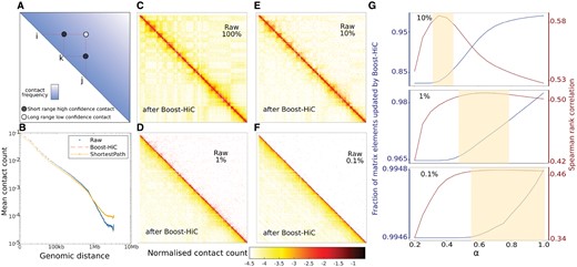
(A) Schematic explanation of our shortest-path enhancement algorithm on Hi-C maps: the low-confidence long-range contact between sites i and j (white dot) is enhanced using the information on shorter-range higher-confidence contacts (black dots) with intermediary nodes (here k). On the contact graph, the shortest path between i and j goes through k, and the enhanced contact value is related to its length. (B) Contact probability curve P(s) of ESCs from their Hi-C map downsampled to 10% of contacts. The blue points display the contact probability curve from the downsampled map. Yellow line displays the curve after information enhancement by means of our shortest-path method. The red line displays the improved contact probability curve at the end of Boost-HiC algorithm, including the step of re-normalization. (C)–(F) Panels display SCN-normalized contact maps (mESC, for a region on chromosome 16 located between 100 kb and 29.8 Mb) at different downsampling ratios: 100, 10, 1 and 0.1% of contacts retained. The SCN normalization applied with the L1 norm ensures that the sum of each line and column is converging to one. The same colour map can be used for all maps. Upper triangular parts display the raw contact map at different downsampling ratios. Lower triangular parts show the map improvement after implementation of Boost-HiC. Colourmap in log10 scale. (G) Spearman rank correlation (in red) between the initial contact map (100%) and downsampled-then-enhanced maps for different downsampling ratios, as a function of the parameter a used in Boost-HiC algorithm. The blue line shows the fraction of updated elements between the downsampled map and the boosted map. From top to bottom, we consider downsampling to 10, 1 and 0.1% of the initial contacts. The shaded beige regions, manually determined, emphasize the optimal ranges for α. (Color version of this figure is available at Bioinformatics online.)

2 Materials and methods

2.1 Hi-C sequence alignment

We used a previously published dataset (Bonev et al., 2017) from mouse embryonic stem cells (ESCs) and cortical neurons (CN) available as GSE96107. Hi-C reads were processed using the mm9 reference genome with HiC-Pro (Servant et al., 2015). Bowtie2 (Langmead and Salzberg, 2012) was used with default pipeline parameter—very-sensitive -L 30 –score-min L,-0.6,-0.2 –end-to-end –reorder. We analyzed replicates for each dataset at a resolution of 10 kb separately, before merging them at the end of the HiC-Pro pipeline. This merged array defines the raw contact map, M.

2.2 Hi-C filtering

The finite experimental resolution amounts to discretize the genome into bins of size equal to the resolution. For each bin, the number of contacts involving a genomic locus in the bin was computed, henceforth termed the contact count of the bin. Hi-C maps were then filtered in two steps. First, bins with vanishing contact counts were removed. In a second step, the distribution of non-zero contact counts was fitted using a Gaussian Kernel Density function (Pedregosa et al., 2011) with parameter kernel=‘gaussian’, bandwidth = 2000. Since Gaussian Kernel Density function returns the logarithm of the distribution, we took the exponential of the output. The resulting distribution was then used to identify bins for which the contact count has a value below 5% and above 95% of the mean contact count. These bins were removed from the contact map. Filtered datasets were finally normalized using the Sequential Component Normalization (SCN, Cournac et al., 2012) so that the L1-norm of each column/line =1. The component C_ij of the resulting SCN-normalized matrix, henceforth termed the normalized contact count, is the conditional probability that the fragment i establishes a contact with fragment j given that it establishes one contact. Note that this normalization produces contact maps that can be compared and plotted with the same colour-scale.

2.3 Contact probability curve

The contact probability curve P(s) as a function of the genomic distance s is computed as the mean normalized contact count along the secondary diagonal located at a distance s from the main diagonal. Since there are less contacts between bins which are more distant along the genome than between closer ones, contacts are averaged over a number of diagonals that increases with s according to a geometric progression (log-binning) of scale factor 1.01. When necessary, we denote $P_C(s)$ the contact probability curve associated with the (normalized) contact map C.

2.4 Boost-HiC implementation

Boost-HiC algorithm operates in several steps. The initial normalized contact map C is first transformed element-wise into a preliminary distance matrix d^o as described in Lesne et al. (2014):

$$d_{ij}^o={(C_{ij})}^{-\alpha }$$

where α is a tunable exponent. This preliminary distance matrix suffers from two major drawbacks. First, since the majority of contact counts in the matrix C are zeros, the matrix d^o contains many undefined elements. Second, calling it a distance matrix is improper in the sense that its elements do not necessarily satisfy the triangular inequality (see Supplementary Fig. S1A). For these two reasons, a shortest-path algorithm (Floyd, 1962) is then run on d^o to get a bona fide distance matrix d. The distance d_ij between any pair of loci i and j is defined as the length of the shortest path connecting them on the weighted contact graph, in which each edge of the graph is given a length equal to the d^o—distance between its ends (Morlot et al., 2016). The resulting matrix d contains elements which are now all defined, non-zero and fulfilling the triangular inequality (see Supplementary Fig. S1B). This complete distance matrix d is then turned element-wise into a densely filled contact map F^o according to the formula:

$$F_{ij}^o={(d_{ij})}^{-1/\alpha }.$$

This formula is the inverse of the formula used to compute the preliminary distance matrix d^o from the normalized contact counts. It thus restores quantities with a similar meaning, while now giving non-vanishing values to elements equalling zero in the matrix C. The same value of α is used in the full range of genomic distances in order to minimize the number of tunable parameters. The number of updated elements, N_r, is computed by counting the number of elements (i, j) which have not the same value in C and F^o. In order to optimize the value of the α exponent, we started with a small value (e.g. 0.05) and then increased this value by step of 0.01 and computed N_r. When N_r started to increase, meaning that we start to spuriously change non-zeros values of the initial contact map (see Fig. 1G), we stopped the procedure and kept this value for the exponent α.

Since the contact probability P(s) as a function of the genomic distance s may change between C and F^o, we have to re-adjust the contact matrix so that the contact probability curve matches exactly the one computed for C. To do so, each contact $F_{ij}^o$ for bins i and j separated by a genomic distance $s=|i-j|$ is multiplied by the ratio $P_C(|i-j|)/P_{F^o}(|i-j|)$ (see Fig. 1B). The final matrix is SCN-normalized at the end of the process to ensure that the sum of lines/columns =1, yielding normalized contact counts.

The code implementing Boost-HiC for a given value of α is available at https://github.com/LeopoldC/Boost-HiC.

Note that the step of dimensional reduction currently involved in 3D chromosomal reconstruction methods [e.g. in ShReC3D Lesne et al. (2014) or BACH Hu et al. (2013)] is not included in Boost-HiC, since it would result in a loss of information. Adapting Boost-HiC procedure to another reconstruction method than ShReC3D, e.g. BACH, would require to carefully dissect the original algorithm in order to exclude the reduction step.

2.5 HiCPlus implementation

HiCPlus has been used as described in Zhang et al. (2018). We modified the original code in order to apply the algorithm to the whole contact map whereas it was originally developed to enhance short-range contacts only. The version of the code we used is available at https://github.com/jbmorlot/HiCPlus/.

2.6 Downsampling

In order to quantify the efficiency of our algorithm, we tested whether it is capable of inferring the full information available in a deeply-sequenced contact map, from a map with less contacts. To implement this test, we sampled the raw contact map using a binomial probability. For every couple of bins i and j, the number of contacts M_ij between these two genomic regions in the raw map is replaced with a random number generated from a binomial distribution of parameters M_ij and k. We successively used three different values of k: 0.1, 0.01 and 0.001, corresponding respectively to downsampling the raw map to 10, 1 and 0.1% of the contacts. This parameter k, controlling the percentage of contacts retained, is henceforth termed the downsampling ratio.

To validate our downsampling method, we used raw reads from ESCs replicate 4. We use two different downsampling procedures: either by using the read sampling programme seqtk (Li, 2018) before running the mapping procedure, or directly on the contact counts obtained after mapping as described above (Supplementary Fig. S2). Resulting contact maps were compared with the original map using both eigenvector similarity (see below compartment determination) and Spearman rank correlation (Supplementary Fig. S3A and B). We also confirmed that the slope of the contact probability curve P(s) is sensitive neither to the downsampling strategy nor to the downsampling ratio, which only affects the level of its fluctuations at large genomic distance (Supplementary Fig. S3C and D).

2.7 Compartments and TADs

Compartments were obtained as in Lieberman-Aiden et al. (2010). First, SCN-normalized contact maps were transformed component-wise to their observed/expected ratio, i.e. each component is divided by the average over the diagonal line to which it belongs. Correlation maps were obtained by computing the correlation between the lines of these transformed matrices, namely the (i, j) component of the correlation map is defined as the correlation between lines i and j. The sign of the components of the first eigenvector of the correlation map was used to infer two compartments, one comprising the bins for which the eigenvector components were positive, the other the bins for which the components were negative. Which one is the A compartment (active compartment) was settled by computing the gene density in each compartment and assigning the label A to the highest-density compartment, the other one being the inactive B compartment.

To infer the position of TADs borders, we computed a TAD border score for each position p along the genome, with a resolution of 10 kb. This score is obtained by summing the contact map elements over a square region of size h with its lower-left corner located on the main diagonal, at the position p. We plotted the TAD border score along the genome by sliding the square along the diagonal of the contact map (Kruse et al., 2016). We chose here a size h of 300 kb. Local minima of this score determined the TAD borders (Smith et al., 2016). Similar TAD borders were obtained using two other state-of-the-art methods: the Insulation score method (Crane et al., 2015) and TopDom (Shin et al., 2016) (Supplementary Fig. S4).

3 Results and discussion

3.1 Boost-HiC partially restores the resolution of downsampled contact maps

Hi-C datasets are generally processed in the form of contact maps, in which the component associated to a pair of loci is determined by normalizing the number of times they have been found together in the Hi-C library, henceforth termed the normalized contact count (Cournac et al., 2012). At fine resolution, i.e. when contacts are summed over small genomic regions (‘bins’), this number is frequently =0 due to the finite sequencing depth. The issue is currently circumvented by working at a lower resolution, by aggregating the restriction fragments into larger and less numerous bins. We propose a computational alternative, Boost-HiC, to infer the missing fine-resolution contact counts from the knowledge of the measured contacts, and get a complete fine-resolution contact map. The procedure is based on the computation of shortest paths between any pair of genomic loci on the contact network, a method that we introduced previously for 3D reconstruction (Lesne et al., 2014; Morlot et al., 2016). More precisely, we first compute the contact probability P(s) as a function of the genomic distance s between two loci, for the normalized contact map C. We also transform the contact map, with elements C_ij, in a distance map with elements

$$d_{ij}^o={(C_{ij})}^{-\alpha }$$

where the exponent α is a parameter to be later optimized. The same value of alpha is used in the full range of genomic distances to minimize the number of tunable parameters. This initial distance map d^o is used to define a weighted contact network, where the link between the loci i and j is given a length $d_{ij}^o$⁠. We then compute an updated distance map using a shortest-path algorithm: the distance d_ij between any two loci i and j is set to the minimal distance between nodes i and j, i.e. the length of the shortest path relating i and j on the contact graph. In this way we get a full distance map d with finite elements d_ij, even when the measured contact frequency between the loci i and j vanishes. This distance map is then converted into a contact map F^o by inverting the above relation element-wise, namely $F_{ij}^o={(d_{ij})}^{-1/\alpha }$⁠. Since short-range contact values are often used to infer longer-range contact values, the contact probability curve may have changed after the procedure. A proper element-wise rescaling of F^o restores the original contact probability curve P(s) (see Section 2 and Fig. 1B). The resulting map is finally normalized using the SCN procedure (Cournac et al., 2012) to give the final ‘boosted’ contact map F. This map F lies at the same fine resolution than the original one, but originally vanishing elements are now replaced with their inferred values.

To assess the capabilities of our algorithm, we generated three contact maps downsampled to 10, 1 and 0.1% of the initial contacts, from a high-resolution contact map of a region of mouse chromosomes 12, 16 and 19 at 10 kb resolution (see Section 2). As expected, as the downsampling ratio increases, more and more matrix elements become =0 in the downsampled matrix (Fig. 1C–F, upper triangles). We then constructed the corresponding boosted maps (Fig. 1C–F, lower triangles). In order to quantitatively compare the boosted maps and our objective, i.e. the original high-resolution version, we computed the Spearman rank correlation between the boosted maps and this original map, as a function of the tunable parameter α. While some other methods have been developed to compare contact maps from different origins (Sauria et al., 2015; Yang et al., 2017), this straightforward measure is apt to compare downsampled maps with the original one. We found that the downsampled maps displayed a reduced Spearman rank correlation of 0.51, 0.26 or 0.11 for downsampling ratios =10, 1 or 0.1%, respectively. This correlation drop was found to be less dramatic when using Pearson correlation, with values of 0.91, 0.83 or 0.34, respectively. The reason for this discrepancy is that Pearson correlation is mainly driven by the high contact count values found close to the diagonal, while being quite insensitive to variations in the lower counts corresponding to long-range contacts. In contrast, the Spearman rank correlation gives a similar importance to all the elements of the contact map and is therefore a better choice (Yang et al., 2017). We then applied Boost Hi-C to the downsampled maps and found an important increase in Spearman rank correlation when α is chosen between 0.51 and 0.59 for the boosted maps obtained from the map downsampled to 10% of the contacts, between 0.26 and 0.51 for a downsampling ratio of 1%, and between 0.11 and 0.47 for a downsampling ratio of 0.1%, as shown on Figure 1G. Pearson correlation remained =0.94, or increased from 0.86 to 0.90 and from 0.51 to 0.76, respectively.

In comparison, HiCPlus (Zhang et al., 2018), which relies on a deep-learning approach where contacts are enhanced using the information contained in the contacts established by the adjacent sites along the genome, achieves Spearman rank correlation values of 0.59, 0.44 and 0.34. Boost-HiC thus offers a better improvement in this case. HiCPlus was specifically designed for enhancing short-range contacts, whereas Boost-HiC mostly improves low-count elements corresponding to long-range contacts. To illustrate this behaviour, we computed the Spearman rank correlation between the diagonal lines of the original full map and the downsampled maps before and after application of Boost-HiC, as a function of the genomic distance (recalling that the distance between a diagonal line and the main one is precisely the genomic distance). While the correlation between the full map and raw downsampled maps continuously decreases with increasing genomic distance, boosted maps display a higher correlation with the full map for intermediate genomic distances and an improved correlation at long ranges (Supplementary Fig. S5).

3.2 Optimizing the parameter α

The different values of the Spearman rank correlation obtained at increasing values of the tunable parameter α showed that unless α is chosen below 0.1 or above 1, the choice of its value has a mild effect on the enhancement efficiency, e.g. Spearman rank correlation changes from 0.53 to 0.58 for a downsampling ratio of 10%, Figure 1G. The value of α yielding the most accurate recovery of the initial map =0.25, 0.5 and 0.6 for downsampling ratios =10, 1 and 0.1%, respectively, hence it is not obvious to assess the value to be used in a practical case. The range of optimal values for α increases when the sequencing depth decreases (mimicked here by decreasing the downsampling ratio). For low α values, only vanishing elements of the downsampled matrix are changed into non-zero values in the boosted matrix (Supplementary Fig. S6). When α increases, the number of matrix elements that are updated by Boost-HiC procedure increases and non-zero elements (close to the diagonal, corresponding to short-range contacts) are also modified. In order to see whether the optimal value for α depends on this number of updated elements, we plotted the number of matrix elements that are reassigned as a function of α value for three different downsampling ratios (10, 1 and 0.1%). This analysis showed that for all three downsampling ratios, the optimal value of α corresponds to the updating of vanishing elements only, i.e. all the zeros and few non-zeros elements (Fig. 1G).

This gives a way to choose an optimal α value in real cases, where we have only access to sparse data. We therefore implemented a search procedure for the optimal α, which corresponds to a re-assignment of all the zeros and 10% of the non-zeros elements only. Since this optimization step for α can be long for large matrices, we propose in this case to estimate the optimal α based on the sparsity of the matrix. For low-sparsity maps (i.e. lower than 0.9) an α value of 0.25 works well whereas for high-sparsity maps (i.e. higher than 0.99) α should be chosen close to 0.6. For intermediate sparsity values, α should be taken between those two bounds.

3.3 Boost-HiC enables the precise determination of compartments from low-resolution maps

As the contact patterns vanish in downsampled maps (Fig. 1C–F), the detection of A/B compartments using the state-of-the-art procedure is accordingly impaired. At a downsampling ratio =0.1%, compartments cannot be identified anymore (Fig. 2A). When the Boost-HiC procedure is applied to the downsampled maps, the detection of these structural features is restored, showing the ability of our computational strategy to reliably detect 3D features from sparse data (Fig. 2B). The algorithm also showed good performance on full chromosome contact maps (Supplementary Fig. S7). Determination of the bins that are more prone to a change in compartment assignment upon downsampling showed that they are usually found in smaller compartments (Supplementary Fig. S8). Using HiCPlus to enhance the downsampled maps also resulted in a partial recovery of the compartments (Fig. 2C). All these results are summarized in Figure 2D, which displays the fraction of bins that are attributed to a correct compartment (i.e. as determined from the high-resolution map), for different downsampling values and enhancement methods. Boost Hi-C robustly allows a better prediction of compartments from low-resolution maps.

Fig. 2.

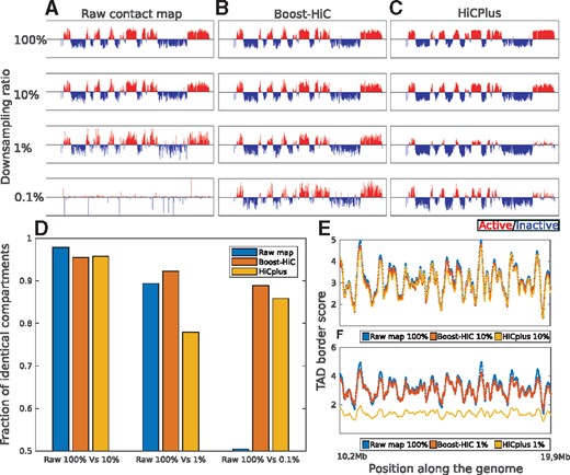
(A) Profile along the genome of the first eigenvector of mouse ESC correlation map, for a region on chromosome 16 located between 100 kb and 29.8 Mb, at different downsampling ratios: 100, 10, 1, 0.1% (from top to bottom). (B) Similar profiles computed after application of the Boost-HiC algorithm. (C) Similar profiles computed after application of HiCPlus algorithm (Zhang et al., 2018). (D) Fraction of genomic regions attributed to the correct compartment, i.e. the compartment derived from the initial map (100%), when starting from downsampled maps, without enhancement (raw maps) or using different enhancement methods, for downsampling ratios =10, 1 and 0.1%, as indicated below the barplot. (E) TAD border score along the genome (from 13.98 to 24.35 Mb on chromosome 16). The blue line displays the score obtained for the initial contact map, i.e. comprising 100% of the contacts. Red and yellow lines correspond to the contact map downsampled to 10% enhanced with Boost-HiC and HiCPlus methods, respectively. (F) Same as panel (E) for a downsampling ratio of 1%. (Color version of this figure is available at Bioinformatics online.)

We took further advantage of our downsampling methodology to compute the finest resolution that can be achieved in determining compartments, given the total number of reads in a chromosomal contact map (Supplementary Fig. S9). Our results on chromosome 19 showed that without Boost-HiC, even a resolution of 100 kb cannot be attained with 10⁵ contacts, whereas compartments can be efficiently determined at 40 kb with a similar number of contacts after application of Boost-HiC (Supplementary Fig. S9C and D).

On the other hand, as TADs are determined from short-range contacts, the TAD border score is not (or very mildly) modified by Boost-HiC procedure, hence TAD detection is not affected (Fig. 2E). In contrast, HiCPlus does change the signal at short scales but the positions of TAD borders given by the minima of the TAD border score are still properly recovered.

3.4 Boost Hi-C enables high-resolution comparison between contact maps

We finally assessed the performance of Boost-HiC procedure for comparing contact maps obtained in different biological conditions. The comparison is usually done by computing the element-wise log-ratio of two such maps. In order to be informative, this comparison could only be done at a resolution for which the signal-to-noise ratio is high. On Figure 3, we compare two contacts maps from two different cell types, mouse ESCs and CN (see Materials and Methods), at different sequencing depths, with and without using Boost-HiC. These maps represent only a sub-region of mouse chromosome 16, however many pairwise contacts between 10 kb bins are equal to 0 in in a typical Hi-C experiment, even at the highest coverage (Fig. 3A). When computing the log-ratio, these elements of the ratio map will therefore be undefined, as they will be equal to ± infinity (in green and yellow on Fig. 3, left panels). In contrast, when the maps have been complemented with Boost-HiC prior to this differential analysis, these elements are now endowed with a finite value (in red and blue on Fig. 3, right panels). As can be expected, this improvement is even more pronounced at low resolution (e.g. at 10% downsampling in Fig. 3B).

Fig. 3.

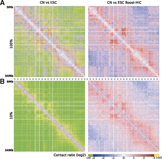
Comparison of contact maps of CN and ESCs. The figure displays the log₂-ratio between CN and ESC contact maps, before (left panels) and after (right panels) application of Boost-HiC procedure. A null element in one map will give an infinite value in the log₂-ratio. (A) Log₂-ratio for maps without downsampling. (B) Log₂-ratio for maps downsampled to 10%

4 Conclusion

Boost-HiC is an efficient computational method to enhance low-resolution chromosomal contact maps. The resulting maps give a high-resolution access to chromosomal compartments. Boost-HiC procedure also improves the identification of differential contacts between two conditions.

Funding

This work was supported by the programme InFIniTI 2018 of the Mission for Interdisciplinarity of the French Centre National de la Recherche Scientifique [grant 238301 to A.L.); the Cancéropôle Grand-Sud-Ouest, programme Emergence 2018 [grant 2018-E08 to A.L.]; and the Agence Nationale pour la Recherche [HiResBac, grant ANR-15-CE11-0023-03 to J.M.].

Conflict of Interest: none declared.