Promoter analysis and prediction in the human genome using sequence-based deep learning models

Abstract

Motivation

Computational identification of promoters is notoriously difficult as human genes often have unique promoter sequences that provide regulation of transcription and interaction with transcription initiation complex. While there are many attempts to develop computational promoter identification methods, we have no reliable tool to analyze long genomic sequences.

Results

In this work, we further develop our deep learning approach that was relatively successful to discriminate short promoter and non-promoter sequences. Instead of focusing on the classification accuracy, in this work we predict the exact positions of the transcription start site inside the genomic sequences testing every possible location. We studied human promoters to find effective regions for discrimination and built corresponding deep learning models. These models use adaptively constructed negative set, which iteratively improves the model’s discriminative ability. Our method significantly outperforms the previously developed promoter prediction programs by considerably reducing the number of false-positive predictions. We have achieved error-per-1000-bp rate of 0.02 and have 0.31 errors per correct prediction, which is significantly better than the results of other human promoter predictors.

Availability and implementation

The developed method is available as a web server at http://www.cbrc.kaust.edu.sa/PromID/.

1 Introduction

The high fidelity of the RNA polymerase II (pol II) transcription system is necessary for precise spatiotemporal regulation of endogenous protein expression and essential to proper development and homeostasis in eukaryotes. Among the key cis-regulatory modules for RNA pol II-mediated transcription is the core promoter, which is typically situated within a DNA segment spanning from −40 to +40 bp relative to the transcription start site (TSS) at position +1 (Danino et al., 2015; Kadonaga, 2012; Vo Ngoc et al., 2017a). This stretch of DNA serves as a platform on which RNA pol II and a number of auxiliary factors assemble into the transcription machinery, which is capable of integrating a range of intrinsic and extrinsic signals, to ultimately determine the proper initiation of transcription (Butler and Kadonaga, 2002; Juven-Gershon et al., 2008; Kadonaga, 2012; Lodish et al., 2000; Morris et al., 2004; Roy and Singer, 2015; Vo Ngoc et al., 2017b; Zabidi et al., 2015). Thus, the characterization of the structure-function relation of the core promoter is crucial to unraveling the complex molecular control mechanisms underlying not just the constitutive basal expression but also the regulated expression in the RNA pol II transcription system.

Decades of in vitro research has identified a number of functional sequence motifs for the RNA pol II core promoter (Butler and Kadonaga, 2002; Roy and Singer, 2015; Smale and Kadonaga, 2003; Vo Ngoc et al., 2017b). Among such functional core promoter elements, perhaps, the most well-known is the TATA-box, which was, in the past, thought to be universally present in RNA pol II core promoters (Vo Ngoc et al., 2017b). However, the advent in genome-wide TSS detections based on high-throughput sequencing revealed that the core promoter structure is highly diverse and complex, and there are no universal core promoter elements (Arnold et al., 2017; Kadonaga, 2012; Lenhard et al., 2012; Roy and Singer, 2015; Vo Ngoc et al., 2017b; Zabidi et al., 2015). Indeed, recent estimates showed that only about 17% of eukaryotic core promoters contain the TATA-box (Yella and Bansal, 2017). More surprisingly, genome-wide structural analysis found that many core promoters do not possess any of the known core promoter elements. Such structural heterogeneity permits the core promoter to expand its functional repertories so as to serve as gene- and cell-type-specific transcription regulator that responds to a range of conditions; however, because of this large diversity, the design principle of the core promoter still remains largely elusive (Arnold et al., 2017; Garieri et al., 2017; Roy and Singer, 2015; Vo Ngoc et al., 2017b).

The structure of the human promoter is notoriously complex and diverse. One explanation for this is that such complex and diverse structures must be ‘designed’ to properly control expression of ∼25 000 protein coding genes based on interactions with only ∼1850 transcription factors in the human genome (Maston et al., 2006). Another explanation comes from a molecular evolution study which discovered substantially accelerated rates of evolution in primate promoters compared with other mammalian promoters (Taylor et al., 2006). This rapid primate promoter evolution was found to be comparable to the neutral substitution rate, suggesting that primate promoters have weak selective constraints, and this suggestion can also explain highly complex and diverse structures in the human promoter. In any case, a better understanding of the structure-function relation of the human promoter has particularly important implications as some genetic variants in such non-coding regions are associated with rare Mendelian diseases (Edwards et al., 2013; Rojano et al., 2018). Furthermore, some cancer cells are associated with somatic mutations in promoter regions (Fredriksson et al., 2017; Vinagre et al., 2013). In order to gain insights into what types of genetic variations can cause aberrant expression leading to human diseases, it is crucial to accurately predict the locations of human promoters and to understand their structural patterns.

Here, we introduce DeeReCT-PromID, a novel machine learning-based approach for the prediction of human RNA pol II core promoters. Taking advantage of the big promoter collection with experimentally validated TSSs (Dreos et al., 2017) generated by modern high-throughput techniques, we build a deep learning model using sequence data as an input. To avoid bias based on prior knowledge about promoter loci (e.g. sequences with known core promoter elements and high density of CpG dinucleotides), we do not use pre-defined features; but rather attempt to discover sequence features and learn salient patterns of the human promoter solely from the training set. This is important especially in the prediction of human promoters since the structural features of many promoters are still unknown (Maston et al., 2006; Roy and Singer, 2015). We previously developed a similar convolutional neural network (CNN)-based algorithm for the prediction of core promoter locations in several model organisms (Umarov and Solovyev, 2017). While this method was able to outperform previously developed promoter prediction methods (Umarov and Solovyev, 2017), its false-positive rate was not adequate enough to ensure the accurate detection of promoters on long genomic sequences. DeeReCT-PromID was developed to chiefly alleviate this limitation and to focus on the promoter prediction on longer sequences. Specifically, to reduce the false-positive rate, we adaptively and iteratively train the predictor by changing the distribution of samples in the training set based on the false-positive errors it made in the previous iteration. By including difficult non-promoter sequences in the training set, we can force the predictor to learn promoter patterns to rule out such sequences. To evaluate the performance of the new method, we compared our method with publicly available tools for the human promoter prediction task. We found that DeeReCT-PromID outperformed the other predictors and achieved a much smaller error-per-1000-bp rate. Our results demonstrate the usefulness of the proposed method for the human promoter prediction on long genomic sequences and suggest its potential value as a tool to gain insights into the design principle for the human core promoters.

2 Materials and methods

2.1 Datasets

Our models are trained using human promoter sequences extracted from the EPDnew database (Dreos et al., 2017). The EPD database is an annotated non-redundant collection of eukaryotic POL II promoters, for which the TSS has been determined experimentally. The authors of the EPDnew database have demonstrated its higher quality over the ENSEMBL-derived (Aken et al., 2016) human promoter set (Dreos et al., 2013).

In this study, we downloaded 16 455 genomic sequences (from −5000 to +5000 bp, where +1 is a TSS position) containing human promoters from the EPD database. We used 90% of the sequences for training and 10% for testing. Positive and negative sets were extracted from the training set. A promoter region of a given size around the known TSS is considered to be a positive sequence. A negative sequence is the one outside the promoter region, which does not contain a known TSS. Initially, the negative set had the same size as the positive one and consisted of randomly picked negative sequences.

2.2 Deep neural network model

We use deep neural networks to identify promoter regions. The data are read in the fasta format and then transformed using one hot encoding. This encoding uses a vector of size 4 to represent each nucleotide. A is encoded as (1 0 0 0), T is encoded as (0 1 0 0), G is encoded as (0 0 1 0) and C is encoded as (0 0 0 1).

Our architecture consists of two CNN which are in parallel (Fig. 1). This means that they both have access to the original input. One CNN has an average pooling layer, while the other does not have any pooling layer. CNN with an average pooling layer has filter length one, while the other one uses filter length 15 and both have two convolutional layers. Average pooling is well suited to capture GC content of the sequence, which is known to be higher in a promoter region (Fenouil et al., 2012), since we only care about the count of G and C nucleotides, not their positions inside a promoter. However, usage of a pooling layer deteriorates positional information which is important for some promoter elements that are located at a specific location in the promoter region, e.g. the initiator (Inr). Using two CNNs in parallel, we solved this conflict and were able to capture various significant promoter features. The outputs of the CNNs are concatenated, flattened and fed into a softmax layer which predicts the probability that an input sequence is a promoter.

Fig. 1.

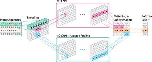
Deep learning model architecture that was used in building promoter models of DeeReCT-PromID (see text for its description)

Weight decay and dropout (Srivastava et al., 2014) are used to improve the generalization capability of our model. Weight decay effectively limits the number of free parameters in the model to avoid overfitting. Introducing weight decay makes it possible to regularize the cost function by penalizing large weights. The main idea of dropout is to randomly set some nodes of the neural network to zero during training to prevent co-dependency among them. During the training we use dropout for the feature vector with keep probability of 0.5. Adam optimization algorithm is used to train the weights (Kingma and Ba, 2014), which is an improved version of stochastic gradient descent. We use TensorFlow (Abadi et al., 2016) as the framework to construct the deep neural network. The training was performed on a workstation with two 980 GTX GPUs and took on average 7 h.

2.3 Classification procedure

We train the model using positive and negative sets which consist of relatively short sequences with a fixed length. As our model accepts sequences of certain length as input we apply a sliding window approach to analyze long genomic sequences. This window is moved across the sequence and at each position the subsequence is fed into our model. The model gives us a score from 0 to 1 that represents the likelihood that a subsequence is a promoter region. If we plot these promoter scores, we will receive a scoring landscape of our model, see Figure 2.

Fig. 2.

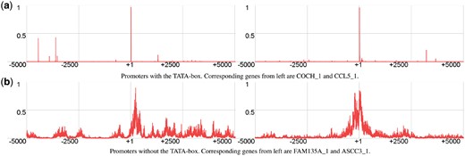
Scoring landscapes constructed by our models. True TSS is at position +1. (a) Promoters with the TATA-box. Corresponding genes from left are COCH_1 and CCL5_1. (b) Promoters without the TATA-box. Corresponding genes from left are FAM135A_1 and ASCC3_1

If the value of the score of a sliding window is above the threshold it is predicted as a start of a promoter region. In practice, we construct two deep learning models—one is for identification of promoter sequences with the TATA-box and one for promoters without it. Promoters can be predicted much more accurately if they have the TATA-box, that is why we firstly apply the model trained specifically for the promoters with the TATA-box (TATA+ model). Next, we apply the model trained with the promoter sequences without the TATA-box (TATA− model). We account the second model predictions that are not too close to the first model predictions. Their output is combined to make the final decision about promoter region position. TSS is then considered to be at a certain position inside the promoter region. For example, if our sliding window has length 600 bp and the positive set was extracted from −200 to +400 bp, then the TSS will be located at position 201 inside the predicted promoter region.

2.4 Negative set construction

When constructing the prediction model to classify promoters we need to choose what sequences to use for non-promoters. This problem is very important because it affects what features our model will use to separate the two classes. For example, suppose we choose random DNA sequences for the negative set. In this case, a very small number of them will have TATA motif at the specific position. Then the neural network model will just use this one feature to achieve almost perfect separation between the two classes. When applying such a model to real world data, the sensitivity will be high however there will be a lot of false positives. Any sequence with a TATA motif at the specific position will most likely be classified as a promoter. Simply increasing the negative set size is not an effective solution as well, because firstly our data becomes unbalanced and secondly, there will be a big chance that neural networks will be stuck at some local minimum as in the case considered above. There are not many sequences in the negative set that will have a good scoring TATA motif, which makes our network likely to derive its recognition model heavily based on this single discriminating feature.

To resolve these issues we propose an iterative approach described below. Firstly, we choose a negative set randomly. Then we repeat the following steps:

1. We train a model with the current negative set.

2. The model is applied to the dataset with long genomic sequences and false positives are recorded.

3. A subset of false positives with the highest scores given to them by the model (the ones that are most similar to the true promoters) from each long sequence are chosen for the new negative set.

4. A new negative set is then constructed by merging the previous one with the new false positives.

This procedure is repeated until there are only a few false positives found processing the training set in Step 2. These steps are illustrated in Figure 3. Such a procedure constructs a difficult negative set which helps to force our neural network to learn deeper and less obvious features to recognize a promoter sequence.

Fig. 3.

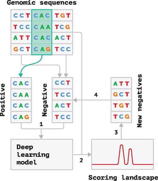
Diagram of our iterative training procedure. See text for the description of each step

2.5 Selecting length and location of input

We need to choose what part of a promoter region to feed into our model for training. In our previous work on promoter identification we used region from −200 to +50 bp to extract promoter features. Since multiple transcription start points (Dreos et al., 2017; Vo Ngoc et al., 2017b) often significantly enlarge potential gene promoter regions, in this work we decided to create a promoter model using a much wider region from −1000 to +500 bp and then apply random substitution procedure to study the location of sequence elements affecting the promoter prediction performance and potentially narrow the region down. The random substitution procedure works as follows. We have a window of size 100, which we move along each sequence with step size 100. At each position we replace the nucleotides with random 100 nucleotides and calculate new promoter score for the modified sequence. The difference between the original score and the new one is recorded and reported for each position (Fig. 4). We noticed that the region from −200 to +400 bp has the most significant effect on the score predicted by our model and this is why it was used to train our final model.

Fig. 4.

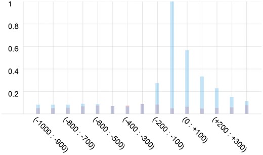
Influence of different regions inside the promoter on the final score produced by the deep learning model. Blue color represents decrease of the score after random substitution and red color shows its increase

2.6 Performance measures

In order to evaluate our method and to objectively compare predictions by our models and the other promoter identification methods, we measured performance using recall, precision, and F1 score:

$$\mathit{Re}call=\frac{\mathit{\text{TP}}}{\mathit{\text{TP}}+\mathit{\text{FN}}},$$

$$\mathit{\text{Precision}}=\frac{\mathit{\text{TP}}}{\mathit{\text{TP}}+\mathit{\text{FP}}},$$

$$F1 \mathit{\text{score}}=2\times \frac{\mathit{\text{Precision}}\times \mathit{\text{Recall}}}{\mathit{\text{Precision}}+\mathit{\text{Recall}}}.$$

If we predict a promoter with the TSS which is closer to the known TSS than the allowed margin for error (500 bp) then this prediction is counted as a TP. If there is no prediction in the area from −500 to +500 bp of the known TSS then we count this case as a FN. Any prediction outside the region from −500 to +500 bp of some TSS is counted as a FP. The same rule is applied for performance evaluation of all the tested promoter prediction programs. Also, we used two accuracy measures that are useful to evaluate the performance of promoter prediction tools when analyzing long genomic sequences: the average prediction error per correctly predicted TSS and the average prediction error per 1000 bp.

3 Results and discussion

3.1 Comparison of predictive performance

We compared our method to all the promoter identification tools we could obtain. A number of promoter prediction methods have been proposed. TSSW (Salamov and Solovyev, 1997) uses a linear discriminant function combining a TATA-box score, triplet preferences around the TSS, hexamer preferences and potential transcription factor binding sites. It has shown good results in a review paper by Fickett (Fickett and Hatzigeorgiou, 1997). FPROM was created by extending the TSSW program feature set, which resulted in significant improvement over TSSW and other promoter recognition software (Solovyev and Shahmuradov, 2003). Promoter2.0 (Knudsen, 1999) extracted promoter elements from DNA sequences and used artificial neuron network to distinguish promoters from non-promoters based on these features. DragonGSF (Bajic and Seah, 2003) also used artificial neuron network as a part of its design and considered GC content and the concept of CpG islands for promoter recognition.

Our previous promoter recognition software, PromCNN achieved good classification performance in discriminating between short promoter and non-promoter sequences (Umarov and Solovyev, 2017). Very recently PromCNN was outperformed by Qian et al. (2018) improving accuracy by about 7%. However, as in Umarov and Solovyev (2017), they focused on the classification performance of short sequences, instead of promoter identification given a long genomic sequence. The latter is a much more difficult problem to tackle because of the high risk of having a large number of false positives. We could not compare our new method to theirs because they did not provide a web server or a tool that would accept long genomic sequences as inputs.

Some of the tools we came across are not available anymore. There are also tools that require extra information besides sequence data as an input. Thus here we compared our method with the following methods: PromCNN, TSSW, FPROM and Promoter 2.0. The results are shown in Table 1. Regardless of the parameters tested, DeeReCT-PromID significantly outperforms the competitors that were examined, which showed relatively good performance in previously published papers (Bajic et al., 2006; Fickett and Hatzigeorgiou, 1997). Our method has F1 score higher than the best competing tool, FPROM, by 0.153. Figure 5 shows an example of the predictions made by the different promoter prediction programs on the sequence containing the promoter of the UBE3D_1 gene. We can see that our method makes no false-positive predictions while still successfully finding the true TSS.

Fig. 5.

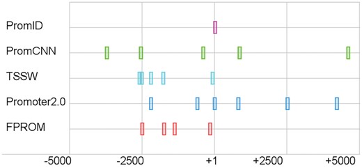
Promoters predicted by the tested promoter identification programs in the DNA sequence of the UBE3D_1 gene. The true TSS is at position +1

Table 1.

Comparison of the performance of the different promoter prediction methods on the test set. Results without marginal predictions (not counting original promoter predictions with low probability) are marked with asterisk

		DeeReCT-PromID	PromCNN	PromCNN*	FPROM	FPROM*	TSSW	Promoter 2.0
Recall	TATA+	0.715	0.884	0.700	0.908	0.647	0.691	0.845
	TATA−	0.745	0.948	0.889	0.868	0.764	0.775	0.810
	BOTH	0.741	0.940	0.865	0.873	0.749	0.764	0.814
Precision	TATA+	0.783	0.118	0.242	0.236	0.491	0.252	0.107
	TATA−	0.758	0.127	0.320	0.227	0.476	0.259	0.104
	BOTH	0.761	0.126	0.310	0.228	0.478	0.258	0.105
F1 score	TATA+	0.747	0.208	0.360	0.375	0.558	0.369	0.190
	TATA−	0.751	0.224	0.471	0.360	0.587	0.388	0.184
	BOTH	0.751	0.222	0.456	0.362	0.584	0.386	0.186
Error per correct	TATA+	0.277	7.464	3.138	3.234	1.037	2.965	8.349
	TATA−	0.320	6.885	2.121	3.403	1.099	2.857	8.581
	BOTH	0.314	6.953	2.225	3.381	1.092	2.869	8.551
Error per 1000 bp	TATA+	0.020	0.660	0.220	0.294	0.067	0.205	0.706
	TATA−	0.024	0.653	0.189	0.295	0.084	0.221	0.695
	BOTH	0.023	0.654	0.192	0.295	0.082	0.219	0.696

Note: The best performance for each measure is in bold.

3.2 Analyzing the learned model

It is well known that the models trained by neural networks are difficult to interpret. We tried to overcome this limitation by visualizing the trained convolutional filters. The maximum filter length we used is 15, thus we decided to find the most important 15-mers identified by our model. We found the top 1000 most influential 15-mers and built a sequence logo for them (see Fig. 6). The top three most important motifs were CCCAGGACCATGTCT, GCTAGGTTGTTATGT, GTTCCCGGCCGGTGC, which all contain GC rich subsequences that are well-known characteristics of eukaryotic promoters (Fenouil et al., 2012).

Fig. 6.

Sequence logo of the most important 15-mers identified by our model

To see the contributions of different nucleotides in different positions of promoter sequences we employed a modification of so called feature mutation map for all sequences in our test set. The mutation maps for TATA+ and TATA− promoters are shown in Figure 7a and b, respectively. To build these maps we took a set of genomic non-promoter sequences with sizes equal to the input sequences used in our promoter models and studied how nucleotide substitutions will change the promoter score computed by our TATA+ and TATA− models. At each position of the tested sequences we replaced a nucleotide with a different one in all these sequences and computed their average promoter score. The rows in Figure 7 represent nucleotides that are used for replacement and the columns show different positions inside the promoter regions. If the new score on average increases it is represented by a red colored square. Decrease of the score is shown by using a blue colored square. The intensity of color is proportional to the effect of substitution on the score. These maps clearly illustrate significant difference of sequence features of TATA+ and TATA− promoters and location of their most conserved elements.

Fig. 7.

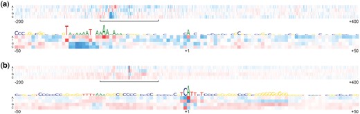
Mutation map for the TSS regions from −200 to +400 bp. Red color represents increase of the score and blue color shows decrease. (a) Model trained on the promoters with the TATA-box. (b) Model trained on the promoters without the TATA-box

We can see that the largest effect on the score in TATA+ model comes from T/A-rich TATA−box region. The most significant element of TATA− promoters is the Inr element, which is very similar to the new consensus sequence for the human Inr core promoter element BBCABW (where, B = C/G/T, W = A/T) described recently in Huang et al. (2017). Such Inr element typically directs the positioning of the transcription initiation start sites representing so called focused promoters in which transcription initiates at a single site or a narrow cluster of sites (Huang et al., 2017). The Inr element contains a conserved motif that is observed in both (TATA+ and TATA−) datasets (see Fig. 8).

Fig. 8.

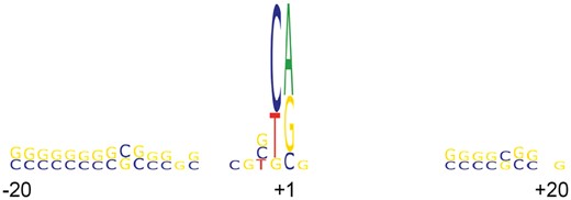
Sequence logo of the region from −40 to +40 bp around the known TSS. The logo demonstrates sequence conservation in the promoter Inr region as well as in two GC rich regions upstream and downstream of TSS

For the TSS position (+1), the most preferred nucleotides are A and G. If a promoter has the Inr element then A is the most frequent nucleotide at position +1, otherwise it is G. This explains why A and G are preferred by our model at position +1 in Figure 7. The sequences at positions −1 to +3 are the most important for setting levels of basal transcription (Kugel and Goodrich, 2017). Changing nucleotides in region −30 to −23 bp from the original ones to G or C reduces the score considerably. While promoter regions in general have more G and C nucleotides, the mentioned region contains TATA-box in TATA+ and tends to have T/A nucleotides in TATA− promoters that is why setting nucleotides to G or C there has a negative effect on the score. In TATA− promoters we also observe occurrence of GC-reach elements (Fig. 7b) that is in agreement with found GC-reach most significant promoter 15-mers described above.

3.3 Accuracy of predictions

As we have shown before, promoters with the TATA-box can be predicted with a very small positional error; often the predicted TSS is exactly at the position of the true TSS. Figure 9 shows distributions of the predictions computed by our method for the test set. High positional accuracy of the TATA promoters is the result of the conserved position of several TATA promoter functional motifs relative to their TSS. However, it is not the case for promoters without the TATA-box for which the predicted positions have a normal distribution around the true TSS. For about 15% of sequences in our test set, predicted TSSs are further than 100 bp from a true TSS. This situation can be partially explained by occurrence of multiple TSSs in non-TATA promoters. Such promoters generate alternative gene isoforms that have tissue or time specific expression. It was shown in Vo Ngoc et al. (2017b) that animal promoters have focused, dispersed and mixed transcription. In dispersed transcription, there are many weak TSSs located at the region from −50 to +50 bp. These multiple TSSs might be responsible for a wide promoter score peak (Fig. 2) for non-TATA promoters generated by our deep learning model. Many of such multiple TSSs as well as some distant alternative TSSs are not annotated in the promoter databases and currently they are considered as false-positives predictions while their actual status requires further experimental verification.

Fig. 9.

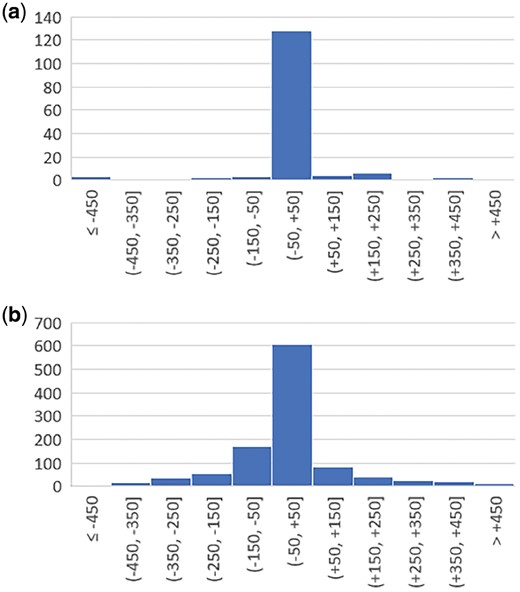
Distributions of predicted TSS positions relative to the annotated TSS for the test set. (a) Model trained on the promoters with the TATA-box. (b) Model trained on the promoters without the TATA-box

4 Conclusion

All computational promoter prediction approaches face complex organization of transcription regulation where a gene may frequently have several promoters, and within one promoter several alternative TSS locations that often are not annotated in promoter databases. All these aspects considerably complicate the development and evaluation of general promoter prediction algorithms. While previously developed promoter prediction methods can relatively accurately classify promoter and non-promoter sequences, they fail to provide good results when applied to study long genomic sequences. Due to potentially huge amount of tested locations they all have very low precision and generate a lot of false positives, which limits their usage in genome-scale studies.

In this work we have proposed a novel training technique to overcome this issue. We used iterative training that focuses on instances that were misclassified by previous iterations and builds our deep learning model that is able to eliminate the huge number of false positives. We analyzed different promoter regions to use as input for feature extraction and chose optimal input location for our tool. Evaluation of our program performance and comparing it to the available promoter prediction tools demonstrated that DeeReCT-PromID significantly outperforms other promoter finding programs.

Many genes have non-coding exons and gene-finders cannot provide the actual gene start and promoter position. Therefore, programs for accurate computational identification of promoters are important for revealing the gene structure and studying gene regulation. This work is a step toward this goal while we understand that this topic is open for further investigations on structure and functioning promoter regions.

Funding

This work was supported by the King Abdullah University of Science and Technology (KAUST) Office of Sponsored Research (OSR) under Awards No. FCC/1/1976-17-01, FCC/1/1976-18-01, FCC/1/1976-23-01, FCC/1/1976-25-01, and FCC/1/1976-26-01.

Conflict of Interest: none declared.