CSHAP: efficient haplotype frequency estimation based on sparse representation

Abstract

Motivation

Estimating haplotype frequencies from genotype data plays an important role in genetic analysis. In silico methods are usually computationally involved since phase information is not available. Due to tight linkage disequilibrium and low recombination rates, the number of haplotypes observed in human populations is far less than all the possibilities. This motivates us to solve the estimation problem by maximizing the sparsity of existing haplotypes. Here, we propose a new algorithm by applying the compressive sensing (CS) theory in the field of signal processing, compressive sensing haplotype inference (CSHAP), to solve the sparse representation of haplotype frequencies based on allele frequencies and between-allele co-variances.

Results

Our proposed approach can handle both individual genotype data and pooled DNA data with hundreds of loci. The CSHAP exhibits the same accuracy compared with the state-of-the-art methods, but runs several orders of magnitude faster. CSHAP can also handle with missing genotype data imputations efficiently.

Availability and implementation

The CSHAP is implemented in R, the source code and the testing datasets are available at http://home.ustc.edu.cn/∼zhouys/CSHAP/.

Supplementary information

Supplementary data are available at Bioinformatics online.

1 Introduction

Inferring haplotype pairs from unphased genotypes is of great importance in genetic analysis. The key point is to solve the phase ambiguity from genotype data, and there have been many methods for haplotype inference (Browning and Browning, 2011; Liu et al., 2008; Niu et al., 2002). Likelihood-based approaches using the expectation-maximization (EM) algorithm and related methods are proved to be statistically efficient under Hardy-Weinberg equilibrium (HWE) (Excoffier and Slatkin, 1995; Qin et al., 2002). On the other hand, a number of Bayesian methods that incorporate complex biological knowledge have been widely studied in literature (Lin et al., 2002; Niu et al., 2002; Stephens et al., 2001; Stephens and Donnelly, 2003; Stephens and Scheet, 2005; Xing et al., 2007; Zhang et al., 2006). Among those, the PHASE algorithm (Stephens and Scheet, 2005) had been considered as a gold standard, in which an approximate coalescent prior was used to model the clustering property of haplotypes. For modern phasing methods, hidden Markov models (HMMs) are often used. Under the assumption that haplotypes tend to cluster into groups over short regions, Scheet and Stephens (2006) proposed the fastPHASE algorithm based on HMM. This algorithm made it possible to a phase larger number of markers and samples. To reduce the computational time of PHASE, Delaneau et al. (2008) used the binary trees to represent the sets of possible haplotypes and proposed a linear complexity phasing method Shape-IT (Delaneau et al., 2011). By combining the local windows approach of phasing in Impute2 (Howie et al., 2011), Delaneau et al. (2013) proposed Shape-IT v2, which has been widely used in the 1000 Genomes Project (Delaneau et al., 2014).

Due to low rates of mutations and re-combinations in genetic evolution and the resultant high linkage disequilibrium (LD) in the genome, only a few haplotypes out of the large number of possible haplotypes are present in population (Daly et al., 2001; Patil et al., 2001). Many algorithms have been developed to maximize different measurements of parsimony of population haplotypes.

Clark (1990) suggested a heuristic approach to reconstruct haplotypes that use the least number of distinct haplotypes. Gusfield (2001) reformulated Clark’s algorithm into a conceptual integer linear programing (ILP) problem, then made a further modification (Gusfield, 2003) to make it practical. Computational results reported that the ILP method is very accurate (Gusfield and Orzack, 2005) for tightly linked polymorphisms. Moreover, Gusfield (2003) proposed an approach to the haplotype inference problem called Pure-Parsimony approach, which tries to find a solution that minimizes the total number of distinct haplotypes used, or equivalently, the ${\ell }_0$ norm of haplotype frequency vector. Unfortunately, the Pure-Parsimony method is NP-hard, which cannot be computed efficiently. Jajamovich and Wang (2012) proposed to obtain a sparse solution by minimizing the Tsallis entropy of the frequency vector, which is still an NP-hard problem.

The most impressive conclusion in compressive sensing (CS) theory in the field of signal processing is that sparse or compressible signals could be accurately and efficiently recovered by minimizing the ${\ell }_1$ norm of signals subject to the measurements from well-behaved under-determined linear sensing systems. Based on this, we propose a regularization algorithm, CSHAP, to reconstruct haplotypes by maximizing an ${\ell }_1$ measure of parsimony defined as the weighted sum of haplotype frequencies, subject to constraints of a series of under-determined linear equations determined by estimated allele frequencies and pairwise covariance (or LD coefficients) of genotypes. Although the use of the first two moments as constraints may lose information, but as we will see later the loss is acceptable and exact or almost exact reconstruction is possible if haplotypes that present in population are sparse.

In this article, we propose a CS framework, CSHAP, for haplotype inference. We first introduce the approach based on the sparse representation of the exact allele frequencies and LD coefficients. Then we relax the constraints by allowing estimation errors in allele frequencies and LD coefficients. We will show that the method is applicable to both individual and pooling designs and works under both HWE and Hardy-Weinberg disequilibrium (HWD). Furthermore, by applying a modified EM algorithm, we can improve the accuracy of the CSHAP algorithm and make it possible to deal with missing data. Finally, based on the idea of partition-ligation (PL) first proposed by Niu et al. (2002), we further extend the algorithm to support long-range haplotypes. Performance of CSHAP is evaluated and compared with other methods by simulation studies and real data analysis.

2 Materials and methods

2.1 Notations

Consider q single nucleotide polymorphism (SNP) loci. Each locus is diallelic and thus theoretically there are $r=2^q$ possible haplotypes. Denote the minor allele at each locus by 1 and major allele by 0. We index the haplotypes by the sequence of coefficients of binary expansion of $0,1,\dots ,r$⁠, i.e. let $h_j=(h_{1j},\dots ,h_{qj})\prime$ represent the jth haplotype vector.

For a specific locus of an individual, if both alleles have a 0 (or 1), this site is called homozygous and is encoded with a 0 (or 2). Conversely, if the two alleles are different, the site is heterozygous and the genotype for the locus is 1. The above encoding also works for pooling designs. Suppose we have T pooled genotype observations at the q loci, each is from a pool of N individuals (or 2N chromosomes equivalently). Let $G_i=(G_{i1},\dots ,G_{iq})\prime$ be the pooled genotypes of the ith pool. Since G_i is a sum of 2N haplotypes, we have $0\le G_{ik}\le 2N,\hspace{0.17em}i=1,\dots ,T,k=1,2,\dots ,q$⁠. If N = 1, then the observations are individual genotypes and T stands for the number of individuals. Our objective is to estimate the haplotype frequencies p based on the genotype observations $G=(G_1,\dots ,G_T)\prime$⁠.

2.2 Sparse representation of haplotype frequency

The minor allele frequency (MAF) for each locus and the joint probability of minor alleles at any two loci can be represented linearly using the haplotype frequencies p. In fact, the MAFs have a linear form representation ${\omega }_0=H\mathbf{p}$⁠, and the joint probabilities of minor alleles can be expressed as ${\eta }_0=H\Lambda H\prime$⁠, where $H=(h_1,\dots ,h_r)$ is a q × r matrix and $\Lambda =\text{diag}\left\{\mathbf{p}\right\}$ is a diagonal r × r matrix with diagonal elements p (Sham et al., 2002). Although η₀ is a matrix consisting of all pairwise allele probabilities of any two loci, i.e. ${\eta }_0{}_{i,j}=\mathbb{P}(\text{locus }i=1,\text{\hspace{0.17em}locus }j=1)$⁠. These two representations are true whether the HWE holds or not. In addition, we have the natural constraint $1\prime \mathbf{p}=1$ since p is a probability distribution. Now we write the above three equations into a single linear equation:

$$\Psi \mathbf{p}=\mathbf{b},$$

(1)

with

$$\Psi =\left(\begin{array}{c}1\prime \\ H\\ H\wedge H\end{array}\right)$$

where the $\frac{q(q-1)}{2}\times r$ matrix $H\wedge H$ denotes the matrix whose rows are the logical product of all pairs of H, and b consists of the scalar 1, the vector ω₀ and vector of the off-diagonal entries of η₀, corresponding to the above three constraints, respectively.

Next, we normalize matrix $\Psi$ such that its columns have unit ${\ell }_2$ norms. Denote ${\Lambda }_{\tau }=\text{diag}({\tau }_1,\dots ,{\tau }_r),$ where τ_j is the ${\ell }_2$ norm of the jth column of $\Psi$⁠. We denote the normalized matrix as $\Phi =\Psi {\Lambda }_{\tau }^{-1}$ and will call it the sensing matrix. Define ${\mathbf{p}}^{*}={\Lambda }_{\tau }\mathbf{p}$⁠. Then (1) can be rewritten as

$$\Phi {\mathbf{p}}^{*}=\mathbf{b}$$

(2)

Note that the sensing matrix $\Phi$ has dimension $\frac{q^2+q+2}{2}\times r$ and the (2) is underdetermined when $\frac{q^2+q+2}{2}<r=2^q$⁠, or equivalently q > 3. Therefore, b can be regarded as the noiseless partial observations of ${\mathbf{p}}^{*}$ from underdetermined linear sensing system $\Phi$⁠.

Because only relatively few haplotypes can be present in a population when the number of possible haplotypes is large, the principle of parsimony has been emphasized in haplotype reconstruction (Clark, 1990; Gusfield, 2003). Noticing the equivalency between the sparsity of p and ${\mathbf{p}}^{*}$⁠, the sparse signal ${\mathbf{p}}^{*}$ can be recovered by solving the following optimization problem:

$$\underset{{\mathbf{p}}^{*}\in {\mathbb{R}}_{+}^r}{\min }\left|\right|{\mathbf{p}}^{*}|{|}_{{\ell }_0}\hspace{0.17em}\hspace{0.17em}\text{subject} \text{to} \Phi {\mathbf{p}}^{*}=\mathbf{b}.$$

(3)

Solving (3) is equivalent to seeking the sparsest solution in the feasible space, which is a combinatorial optimization problem and is NP-hard.

The ${\ell }_1$ norm is known as the convex envelope of the ${\ell }_0$ norm over convex set $\Delta =\{x\in {\mathbb{R}}^r:|\left|x\right|{|}_{\infty }\le 1\}$ when $\left|\right|x|{|}_{\infty }=\max x_i$⁠. In other words, $\left|\right|x|{|}_{{\ell }_1}$ is the best pointwise approximation to $\left|\right|x|{|}_{{\ell }_0}$ among the set of convex function on Δ (Hiriart-Urruty and Lemaréchal, 1993; Recht et al., 2010). Thus, instead of minimizing the ${\ell }_0$ norm of ${\mathbf{p}}^{*}$ directly, we suggest the ${\ell }_1$ minimization:

$$\underset{{\mathbf{p}}^{*}\in {\mathbb{R}}_{+}^r}{\min }\left|\right|{\mathbf{p}}^{*}|{|}_{{\ell }_1}\hspace{0.17em}\hspace{0.17em}\text{subject} \text{to} \Phi {\mathbf{p}}^{*}=\mathbf{b}.$$

(4)

which is the typical form in CS theory and can be solved efficiently by linear programing.

The above Equation (4) is based on known exact value of b, however, b is unknown and needs to be estimated based on genotype observations. In the next subsection, we will make some modifications of (4) by allowing b with estimation errors.

2.3 Presence of noise

The MAFs can be readily estimated by sample means ${\widehat{\omega }}_0={\sum }_i{G}_i/(2NT)$⁠. Under the assumption of HWE, the variance–covariance matrix of the q alleles can be estimated by sample variance–covariance matrix ${\widehat{\Sigma }}_0={\sum }_i{G}_i{G}_i^{\prime }/(2NT)-2N{\widehat{\omega }}_0\widehat{\omega }{\prime }_0$ (Zhang et al., 2008). Then the two-locus joint probabilities ${\eta }_0={\Sigma }_0+{\omega }_0\omega {\prime }_0$ can be estimated by ${\widehat{\eta }}_0={\widehat{\Sigma }}_0+{\widehat{\omega }}_0\widehat{\omega }{\prime }_0$⁠. Then a natural estimate of $\mathbf{b}$ is $\widehat{\mathbf{b}}$ consisting of 1, $\widehat{\omega }$ and the off-diagonal entries of $\widehat{\eta }$⁠.

Now allowing error of $\widehat{\mathbf{b}}$ in measuring $\Phi {\mathbf{p}}^{*}$⁠, we transform the optimization Equation (4) into the following robust problem:

$$\underset{{\mathbf{p}}^{*}\in {\mathbb{R}}_{+}^r}{\min }\left|\right|{\mathbf{p}}^{*}|{|}_{{\ell }_1}\hspace{0.17em}\hspace{0.17em}\text{subject} \text{to}\hspace{0.17em}\hspace{0.17em}||\Phi {\mathbf{p}}^{*}-\widehat{\mathbf{b}}|{|}_{{\ell }_2}\le ϵ$$

(5)

where ϵ is a tuning parameter controlling the error of estimates. This problem is a special case of second order cone programing (Boyd and Vandenberghe, 2004), which can be solved efficiently by many standard approaches such as iteratively reweighted least squares or interior-point algorithms.

The haplotype frequency p_j is then estimated by ${\widehat{p}}_j={\widehat{p}}_j^{*}/{\tau }_j,j=1,\dots ,r,\hspace{0.17em}{\mathbf{p}}^{*}$ is the solution to (5). Necessary normalization is carried out to ensure $\widehat{\mathbf{p}}$ is a proper probability distribution.

2.4 Selection of tuning parameter ϵ

To solve the Equation (5), we need to select a proper tuning parameter ϵ. Given the fact that ϵ = 0 when $\widehat{\mathbf{b}}=\mathbf{b}$⁠, the ϵ should be as small as possible as the ${\ell }_2$ estimation error of the first two moments should not be too large. However, we found that there is usually no solution for (5) if ϵ = 0 as typically $\widehat{\mathbf{b}}\ne \mathbf{b}$⁠. On the other hand, the estimated frequencies are degenerate to $(1,0,\dots ,0)\prime$ as $ϵ\to \infty$⁠.

It is reasonable to believe that, for sufficiently large T and N, the estimates $\widehat{\mathbf{b}}$ is very close to b with certain probability, thereby the level of noise (⁠${\ell }_2$ error of estimates) is bounded. The ϵ should be related to the signal-to-noise ratio, which is directly determined by T, N and b.

From the Central Limit Theorem in statistics, we know that if the pool size N is large, then G_i will be asymptotically normally distributed with mean ${\mu }_G=2N{\omega }_0$ and covariance matrix ${\Sigma }_G=2N{\Sigma }_0$ (Kuk et al., 2008). Using this fact we obtain (Bilodeau and Brenner, 2008)

$$\begin{array}{c}2N\sqrt{T}({\widehat{\omega }}_0-\omega ){\displaystyle \stackrel{d}{\to }}\mathcal{N}\left(0,{\Sigma }_G\right)\\ 2N(T-1){\widehat{\Sigma }}_0{\displaystyle \stackrel{d}{\to }}{\mathcal{W}}_q\left(T-1,{\Sigma }_G\right)\end{array}$$

(6)

Here ${\displaystyle \stackrel{d}{\to }}$ represents convergence in distribution and ${\mathcal{W}}_q(T-1,{\Sigma }_G)$ represent the Wishart distribution with T − 1 degrees of freedom and scale matrix Σ_G.

Denote $e=\widehat{\mathbf{b}}-\Phi {\mathbf{p}}^{*}$⁠, approximately we have $e\sim \mathcal{N}(0,{\Sigma }_e)$⁠, where ${\Sigma }_e=\text{Var}(\widehat{\mathbf{b}})$⁠. Consider the squared norm of the error $\left|\right|e|{|}_{{\ell }_2}^2=e\prime e$⁠, then:

$$\begin{array}{c}\mathrm{E}(e\prime e)=\text{tr} \left({\Sigma }_e\right)\\ \text{Var}(e\prime e)=2 \text{tr} \left({\Sigma }_e{\Sigma }_e\right)\end{array}$$

holds asymptotically. Based on the well-known concentration inequalities, the probability that $\left|\right|e|{|}_{{\ell }_2}^2$ exceeds its mean plus 2 or 3 standard deviations is small (<5 or 2%, respectively). We then solve (5) with

$${ϵ}_{\lambda }^2=\text{tr} \left({\Sigma }_e\right)+\lambda \sqrt{2 \text{tr} \left({\Sigma }_e{\Sigma }_e\right)}$$

and simply select λ = 2.

Since all the components of the vector $\widehat{\mathbf{b}}$ are made up of the elements in ${\widehat{\omega }}_0$ and ${\widehat{\Sigma }}_0$⁠, and we have obtained the asymptotic distribution of them in (6). The variance–covariance matrix Σ_e of $\widehat{\mathbf{b}}$⁠, can be derived or estimated from ${\widehat{\omega }}_0$ and ${\widehat{\Sigma }}_0$ naturally (details can be found in the Supplementary Section 1.1).

2.5 The deviation of HWE

Likelihood-based methods for estimating haplotype frequencies often require the assumption of HWE, but which may not be true if there exists population substructure. Here we introduce the inbreeding coefficient ρ to describe the possible dependence of the two haplotypes within a subject (Zeng and Lin, 2005). The distribution of diplotype $H=[h_k,h_l]$ is assumed as:

$$\mathbb{P}(H|\mathbf{p},\rho )=(1-\rho )p_k{p}_l+\rho p_k{\mathbb{I}}_{k=l},$$

(7)

where ${\mathbb{I}}_{k=l}$ is the indicator of whether k = l. Larger ρ means more similar between H₁ and H₂. Note that if one takes ρ = 0, then this is equivalent to the HWE assumption. Under model (7), the variance–covariance matrix of the genotype data is ${\Sigma }_{\rho }=(1+\rho ){\Sigma }_0=(1+\rho )({\eta }_0-{\omega }_0\omega {\prime }_0)$ which can be estimated by ${\widehat{\Sigma }}_{\rho }=\frac{1}{2NT}{\sum }_i{G}_{i}G{\prime }_i-2N{\widehat{\omega }}_{\rho }\widehat{\omega }{\prime }_{\rho }$ and ${\widehat{\omega }}_{\rho }={\widehat{\omega }}_0=\frac{1}{2NT}{\sum }_i{G}_i$⁠. The joint probabilities ${\eta }_{\rho }$ therefore are estimated by ${\widehat{\eta }}_{\rho }={\widehat{\Sigma }}_{\rho }/(1+\widehat{\rho })+{\widehat{\omega }}_{\rho }\widehat{\omega }{\prime }_{\rho }$⁠, where $\widehat{\rho }$ is an estimate of ρ. In this article, unless when HWE is explicitly assumed, we adopt the following estimate

$$\widehat{\rho }=\frac{{\sum }_{i=1}^q{V}_i}{{\sum }_{i=1}^q{\overline{G}}_i(1-{\overline{G}}_i/2N)}-1,$$

where ${\overline{G}}_i$⁠, V_i is the sample mean and variance of genotypes of ith locus, respectively.

Then b can be readily estimated by the estimator ${\widehat{\mathbf{b}}}_{\rho }=\widehat{\mathbf{b}}\left({\widehat{\omega }}_{\rho },{\widehat{\eta }}_{\rho }\right)$⁠. Now problem (5) is then modified to

$$\underset{{\mathbf{p}}^{*}\in {\mathbb{R}}_{+}^r}{\min }\left|\right|{\mathbf{p}}^{*}|{|}_{{\ell }_1}\hspace{0.17em}\hspace{0.17em}\text{subject} \text{to}\hspace{0.17em}\hspace{0.17em}||\Phi {\mathbf{p}}^{*}-{\widehat{\mathbf{b}}}_{\rho }|{|}_{{\ell }_2}\le ϵ$$

(8)

where ϵ is the ${\ell }_2$ error bound.

On the other hand, introducing a new estimator $\widehat{\rho }$ will increase the variance, especially when ρ gets close to zero. In this case, the departure from HWE is negligible and it is not worth considering an extra inbreeding parameter, since our EM algorithm is relatively robust to deviations from HWE. An adaptive way to test the hypothesis

$$H_0:\rho =0\leftrightarrow H_1:\rho >0$$

(9)

In the simulation experiment, we compute ${\widehat{\rho }}_L=\widehat{\rho }-1.645\sqrt{{\widehat{v}}_{\rho }}$⁠, the 95% lower one-sided confidence bound, where the $\sqrt{{\widehat{v}}_{\rho }}$ is the variance of $\widehat{\rho }$ obtained by bootstrap. If ${\widehat{\rho }}_L>0$⁠, we will use the modified Equation (8). If ${\widehat{\rho }}_L\le 0$⁠, we will ignore the inbreeding parameter and still use (5).

2.6 CSHAP for individual DNA data

For individual genotyping design (N = 1), the Equation (5) can accurately identify the major haplotypes which really exist in the population, but the values may be biased.

Notice that the Equation (5) does not guarantee the compatibility of haplotypes with all the observed genotypes, especially when ϵ is relatively large, while too small ϵ may leads to no solution. Therefore, we first find the smallest ϵ₀ such that solution exists. Then we calculate the largest ${ϵ}_{\lambda }$ described in Section 2.4. Now we have a range of ϵ values $\left[{ϵ}_0,{ϵ}_{\lambda }\right]$⁠. For every ϵ that falls within this interval, our equation will return a series of solutions with different compatibility and sparsity. In all these compatible solutions, we choose the sparsest one as $\widehat{\mathbf{p}}$⁠.

Once we get the above solution $\widehat{\mathbf{p}}$⁠, we obtain a set of haplotypes $\mathcal{H}$ based on the non-zero entries of $\widehat{\mathbf{p}}$⁠. Now we can use $\widehat{\mathbf{p}}$ and $\mathcal{H}$ as the input of the standard EM algorithm. In each iteration, we will only consider the haplotypes contained in $\mathcal{H}$⁠, and only update their corresponding frequencies in $\widehat{\mathbf{p}}$⁠.

In fact, the $\widehat{\mathbf{p}}$ is quite close to the true haplotype frequency, especially for common-frequency (⁠$p_i\ge 5\%$⁠) variants. Correspondingly, $\mathcal{H}$ is very similar to the haplotypes that really present in sample genotypes, so that we can regard $\mathcal{H}$ as a haplotype reference panel. For most individuals, we can find only one compatible diplotype configurations in the reference panel; then, we regard these solutions as ‘solved’ and exclude them in the following iterations. Although most of the phasing algorithm needs to update the estimated haplotypes for every individuals in each iteration, we only consider the remaining ones. Furthermore, when the total number of individuals T is large, we only use the distinctive genotypes that appear in the remaining individuals, since the number of distinctive genotypes is very limited compared with T. These modifications will significantly reduce the number of individuals that need to be considered in each iteration.

Another important feature of our algorithm is that it can deal with missing data easily. We only need to estimate sample moments in Equation (5) based on samples which are complete on the locus or loci involved. The missing locus is then imputed with $\mathcal{H}$ in the subsequent EM procedures (details can be found in the Supplementary Sections 1.2 and 1.3).

The resulting hybrid algorithm, referred as the CSHAP algorithm, incorporates the advantages of both CS theory and EM algorithm. Our algorithm can be more accurate than purely using Equation (5) and more computationally efficient than the current state-of-the-art algorithms.

2.7 CSHAP for large DNA pools

The haplotype estimation methods of pooled DNA data can be divided into two categories: To focus on a small number of pool sizes N (each pool contains about two to three individuals) with large number of markers q, or to consider on a small number of markers q but lager pool sizes N. The former can be solved with EM algorithm (Yang et al., 2003), however, for the other case, the EM algorithm is computationally involved and is not feasible when pool size $N\ge 10$⁠. Kuk et al. (2008) proposed an approximate EM (AEM) algorithm based on Central Limit Theorem, which makes the method based on EM algorithm computationally feasible for large N, with substantial improvement in accuracy simultaneously. However, the time consumption of AEM grows exponentially with q, which limits the performance of AEM when q is larger.

In this case, we substitute the EM procedure in CSHAP with the AEM algorithm. The resulting hybrid algorithm runs nearly two orders of magnitude faster than AEM while exhibiting almost same accuracy.

2.8 CSHAP for long-range haplotypes

Due to the computer memory constraint, our algorithm supports at most 24–27 loci for the length of each block. When the number of loci q exceeds this limit, we apply a special PL strategy (Niu et al., 2002).

Assuming the genotype data consists of $L=K\times M$ loci, where M is the number of blocks and K is the length of each block. Without loss of generality, the genotype data can be divided into M contiguous ‘atomistic’ blocks. In most of the previously published articles (Delaneau et al., 2011; Niu et al., 2002; Qin et al., 2002; Stephens and Scheet, 2005;), K was usually set between 5 and 8 due to the limitation of algorithms. In contrast, our method allows setting K = 16–20 while maintaining efficiency. Obviously, larger K and smaller M can help avoid the local-mode problem (Qin et al., 2002) of EM.

Once we have conducted the CSHAP procedure for each of M atomistic blocks, we iteratively combine the $(2i-1)$th block with the subsequent $(2i)$th block until all blocks are ligated as one. Most of the PL methods usually take D haplotypes with top estimated frequencies in each block, where D can be specified between 40 and 50 (Niu et al., 2002) or be determined separately by some frequency thresholds (Stephens and Donnelly, 2003). This ‘thrown away’ procedure can limit the number of possible concatenated haplotypes to D², but may lead the algorithm to trap into a local mode simultaneously. Here we use all estimated haplotypes in each block instead. However, the total number of all possible concatenated haplotypes may be significantly larger than D². Notice that only relatively few concatenated haplotypes are true among all those possible haplotypes, we use CS again in this ligation step.

Next we demonstrate how to combine the block A with the adjacent block B. From the estimated haplotype frequencies ${\widehat{\mathbf{p}}}_A$ we obtain a haplotype set ${\mathcal{H}}_A$ with n_A haplotypes. Denote $H_A=\left(h_{n_1},\dots ,h_{n_A}\right)$ is a $q_A\times n_A$ matrix obtained by combining the haplotype vectors in ${\mathcal{H}}_A$ by column. Similarly, we have ${\mathcal{H}}_B$ and H_B for block B. Denote the set of all possible concatenated haplotypes as ${\mathcal{H}}_{A\times B}$⁠. Define H_AB is a $(q_A+q_B)\times (n_A{n}_B)$ matrix which can be regard as the Cartesian product of H_A and H_B. Similar to the structure of $\Psi$ in the (1), we have:

$${\Psi }_{AB}=\left(\begin{array}{c}1\prime \\ H_{AB}\\ H_{AB}\wedge H_{AB}\end{array}\right)$$

and ${\Phi }_{AB},{\Lambda }_{AB},{\mathbf{p}}_{AB}^{*},{\mathbf{b}}_{AB}$ correspondingly.

Now we transform the ligation problem into this following problem, which has been already resolved in the above.

$$\underset{{\mathbf{p}}_{AB}^{*}\in {\mathbb{R}}_{+}}{\min }\left|\right|{\mathbf{p}}_{AB}^{*}|{|}_{{\ell }_1}\hspace{0.17em}\hspace{0.17em}\text{subject} \text{to}\hspace{0.17em}\hspace{0.17em}||{\Phi }_{AB}{\mathbf{p}}_{AB}^{*}-{\widehat{\mathbf{b}}}_{AB}|{|}_{{\ell }_2}\le ϵ$$

The non-zero entries of ${\widehat{\mathbf{p}}}_{AB}$ correspond to the estimated haplotypes and frequencies in ${\mathcal{H}}_{A\times B}$⁠. We can also use the EM algorithm to improve the accuracy of ${\widehat{\mathbf{p}}}_{AB}$⁠. This process is repeatable until all blocks are connected as one.

When the number of loci increases to, say, more than 1000s, the frequency estimation is meaningless, since almost every haplotypes are rare. What we actually do at this time is ‘phasing’, which is a totally different task. However, with a few changes, our algorithm can be used as a phasing tool under this situation. We describe the details and results in the Supplementary Section 1.4.

3 Results

We demonstrate the performances of our algorithm by simulations. First we compare the estimation accuracies of CSHAP, PHASE v2.1.1, fastPHASE v1.4, Shape-IT v2.17 and PL-EM v1.0 (with default settings) using individual genotyping data under the assumption of HWE as well as HWD. In addition, we illustrate the computational efficiency of CSHAP in comparison with the others.

For pooling design, we compare the estimation accuracies of CSHAP, PoooL and AEM with various pool sizes and sample sizes. Meanwhile, we show the running time of CSHAP and AEM. All the simulations are repeated 10 000 times if not specified explicitly. Our platform is a desktop computer with Ubuntu 16.04 64-bit, Intel Core i5-7400 CPU@3.00 GHz and 8.0 GB RAM.

To summarize the accuracies of our methods, and to compare the accuracies between the different algorithms, we use two measures: the absolute discrepancy (Excoffier and Slatkin, 1995) and the ${\chi }^2$ distance. The asbolute discrepancy between the estimated haplotype frequencies and their true values is defined as ${\sum }_{i=1}^r\left|{\widehat{p}}_i-p_i\right|/2$⁠, and the ${\chi }^2$ distance is defined as ${\sum }_{i=1, p_i\ne 0}^r{({\widehat{p}}_i-p_i)}^2/p_i$⁠.

3.1 Individual design

We generate T unrelated individual genotypes according to the commonly used 10-locus haplotype frequencies of angiotensinogen (AGT) gene considered in Yang et al. (2003) by assuming HWE, $T=10,20,50,100,200,500,1000,2000$⁠. Part of the results is demonstrated in Supplementary Table S2. We can see that for small sample size, the performances of CSHAP are better than the others in the sense of bias and the effective accumulated probability (EAP) of p. Also CSHAP has smaller estimation bias of almost every haplotype than PHASE’s and Shape-IT’s. For larger sample sizes (⁠$T\ge 100$⁠), the precision of CSHAP is very close to the PHASE and PL-EM, and slightly better than Shape-IT.

Simulation results are summarized in Figure 1. We can see that, for small sample size (T <  100), the absolute discrepancy of CSHAP is smaller than those of the others, and the solution of CSHAP is much sparser than those of PHASE and Shape-IT. When T exceeds about 100, CSHAP behaves as accurate as PHASE, while slightly better than fastPHASE and Shape-IT.

Fig. 1.

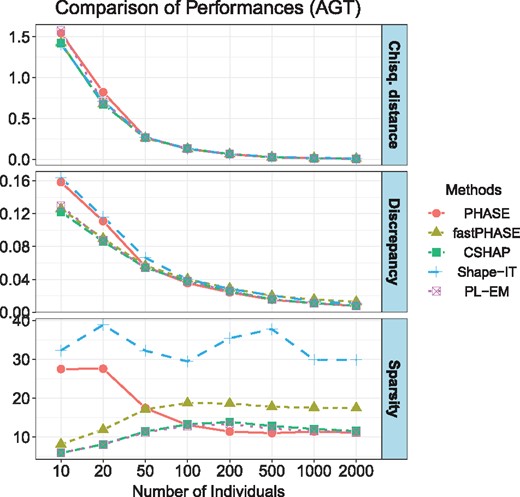
Average accuracy comparison in 10 000 trials with increasing numbers of sample size T. The top panel shows the ${\chi }^2$ distance between the true frequency and estimated frequencies. The second panel shows the absolute discrepancy. The bottom panel shows the sparsity (the number of existing haplotypes in solution), respectively. The true haplotype dataset has 11 unique existing haplotypes

Comparisons of computational efficiencies are given in Table 1. The CSHAP is at least two to three orders of magnitude faster than PHASE and fastPHASE. For T = 100 in our simulation, the CSHAP is 365 times faster more efficient than PHASE while maintaining the same accuracy. For T = 2000, the CSHAP is 1775 times faster than PHASE, 2010 times faster than fastPHASE, 468 times faster than Shape-IT and 19 times faster than PL-EM. Notice that the running time of most other methods shows approximately linear trends with sample size T, and in contrast, our method only in the order of a logarithmic scale. More details are in Supplementary Figure S1.

Table 1.

Running times of CSHAP, PHASE, fastPHASE, Shape-IT and PL-EM algorithm for 1000 replicates of simulation

T	CSHAP	PHASE	fastPHASE	Shape-IT	PL-EM
10	10.2	741	338	120	140
20	12.9	1459	651	139	142
50	17.5	3726	1589	246	146
100	21.1	7727	3145	410	156
200	26.0	9851	6309	731	188
500	29.1	16 619	15 746	2007	258
1000	30.8	28 471	32 019	6014	384
2000	32.6	57 990	65 662	15 318	645

Note: Using Yang et al. (2003)s 10-locus haplotype frequencies of AGT dataset for individual data. The unit of running time is second. T stands for the sample size.

3.2 Haplotype diversity and missing data

To measure the performances under different haplotype diversities, we generate T = 100 individual genotypes according to the 11-locus G6PD haplotypes in Sabeti et al. (2002). The G6PD haplotypes are different among the following six ethnic populations: African American, Asian, Beni (Nigeria), European American, Shona (Zimbabwe) and Yoruba (Nigeria). The published haplotypes and frequencies are given in Supplementary Table S3. In addition, we randomly mask about 5% of the data as missing sites.

As Figure 2 shows, our CSHAP method performs well under varying degrees of diversities, as well as missing data imputation. In fact, the ${\chi }^2$ distances and the absolute discrepancies of PHASE, fastPHASE, CSHAP are similar. The Shape-IT identified too many non-existent haplotypes, which leads to higher discrepancies. PL-EM seems to have problems accurately imputing missing data in the Asian population. Our CSHAP method has almost the same precision as PHASE, while fastPHASE is only a little less accurate than PHASE, but our method gives a sparser solution with the same precision.

Fig. 2.

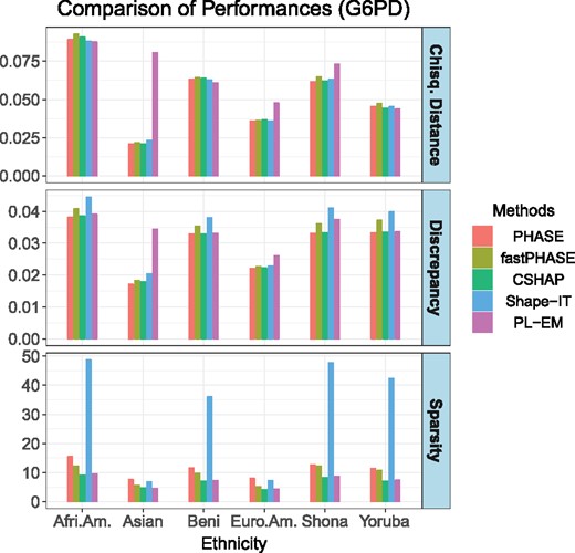
Measures of performance of PHASE, fastPHASE, CSHAP, Shape-IT and PL-EM based on the simulated G6PD gene datasets among six different populations. Sample size T = 100, all the simulations are repeated 10 000 times

3.3 The case of HWD

We generate T = 100 haplotype pairs from (7) using the 10-locus AGT gene with a series of inbreeding coefficients $\rho =0.05,0.1,0.15,0.2,0.3$⁠. For each of 10 000 simulation trials, we first construct a bootstrap sample by resampling with replacement from these sample genotypes 1000 times to estimate the variance of $\widehat{\rho }$ in (9). The proportion of times out of the simulations that ${\widehat{\rho }}_L\le 0$ is $0.888,0.750,0.502,0.303,0.065$⁠, for the above mentioned different values of ρ, respectively.

Results are summarized in the Supplementary Table S4. We can see that introducing a $\widehat{\rho }$ helps to reduce the impact of deviations from HWE, but the SDs are slightly larger. Our adaptive estimator ${\widehat{\rho }}_L$ can make this tradeoff conveniently.

3.4 Pooling design

Next we consider large pooling design. The simulations are based on pooled 10-locus AGT gene data with N = 50, 100 and T = 50, 100 where HWE is assumed. We investigate the performance of CSHAP with PoooL and AEM. To compare with previous published results by Kuk et al. (2008) and Zhang et al. (2008), we use the averaged Euclidean distance $d=\sqrt{{\sum }_{i=1}^r{\left({\widehat{p}}_i-p_i\right)}^2/r}$ instead of ${\chi }^2$ distance.

Figure 3 shows summarized results. The performance of PoooL is not optimal, since the distance and discrepancy are many times higher than those of AEM and CSHAP. Meanwhile, CSHAP shows comparable performance with AEM, the distance and discrepancy are slightly higher, but CSHAP can obtain sparser results than AEM. However, the computational efficiency of CSHAP is about two orders of magnitude faster than that of AEM, Supplementary Table S5 demonstrates that CSHAP runs about 120 times faster than AEM in our simulations.

Fig. 3.

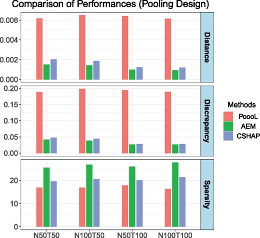
Measures of performance of PoooL, AEM and CSHAP. T stands for the number of pools, and each pool contains N individuals. For each pooling design and method, simulation was repeated 10 000 times

3.5 Long-range haplotypes

In this section, we use the human angiotensin converting enzyme (ACE) dataset. This dataset contains q = 52 SNPs and 11 individuals, the genotypes have up to 37 heterozygous sites. For all individuals, 13 unique haplotypes from the 22 chromosomes are resolved in Rieder et al. (1999). We generate $T=50,100,200,500,1000,2000$ unrelated individual genotypes by assuming HWE and test all the methods in Section 3.1. The result is shown in Figure 4. Our method, PHASE and PL-EM produce the best solution, but CSHAP costs much less time. The biases of Shape-IT and fastPHASE are relatively slightly larger.

Fig. 4.

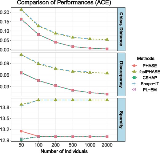
Measures of performance of PHASE, fastPHASE, CSHAP, Shape-IT and PL-EM. For each method and sample size T, simulation was repeated 1000 times. The Shape-IT failed to estimate haplotype frequencies when T = 2000, since the program aborted with an error

The running time of all methods are described in Table 2. CSHAP is about two to three orders of magnitude faster than PHASE and fastPHASE, while providing the most accurate results. For example, when T = 2000, the CSHAP is 3000 times faster than PHASE, 1634 times faster than fastPHASE, 303 times faster than Shape-IT and 10 times faster than PL-EM. More details are in Supplementary Figure S2.

Table 2.

Running times of CSHAP, PHASE, fastPHASE, Shape-IT and PL-EM algorithm for 100 replicates of simulation

T	CSHAP	PHASE	fastPHASE	Shape-IT	PL-EM
50	9.5	4706	821	98	63
100	9.7	9571	1684	228	84
200	10.9	12 176	3324	457	93
500	12.0	19 687	8283	1196	107
1000	14.1	33 783	16 477	3250	140
2000	20.2	60 690	33 083	6153	211

Note: Using Rieder et al. (1999)s 52-locus haplotype frequencies on ACE dataset. The unit of running time is second. T stands for the sample size.

4 Conclusion

In this study, we propose an efficient algorithm, CSHAP, for estimating haplotype frequencies from individual or pooled DNA data, under the HWE assumption or not. The CSHAP algorithm minimizes the weighted sum of haplotype frequencies under constraints on the allele frequencies and covariances (i.e. LD coefficients). This method is based on the maximum parsimony principle of Gusfield (2003), which was to minimize the total number of distinct haplotypes, subject to the condition that the solutions are consistent with genotype observations. In our approach, we substitute the ${\ell }_0$ norm by the ${\ell }_1$ norm and reduce the consistency condition to a system of linear constraints on the first two moments of genotype observations. Besides, we use a modified EM algorithm to boost accuracy efficiently.

Extensive simulation studies show that our method is comparable to or better than the existing methods but has significant computational advantage. An outstanding feature of our method is its computing efficiency for both individual and pooled DNA data. We showed that if the number of existing haplotypes in population is small, our method can recover the haplotypes with high accuracy. In addition, by introducing the inbreeding coefficients the HWE assumption is not required in our approach and this quantity can also capture the inflation of variance in genotype observations caused by genotype errors, population substructures etc.

Furthermore, by introducing the divide-and-conquer idea of PL, our method is able to handle long-range haplotypes. The specially designed PL algorithm can help us to overcome the local-mode problem while maintaining efficiency. In conclusion, our method can be a powerful and efficient approach in genome-wide association studies.

Acknowledgements

We appreciate the insightful comments and helps from Dr Xing Hua and Dr Yifang Yang during preparation of this article.

Funding

This work has been supported by the National Science Foundation of China [NSFC 11671375 and 11271346].

Conflict of Interest: none declared.