SUBSTRA: Supervised Bayesian Patient Stratification

Abstract

Motivation

Patient stratification methods are key to the vision of precision medicine. Here, we consider transcriptional data to segment the patient population into subsets relevant to a given phenotype. Whereas most existing patient stratification methods focus either on predictive performance or interpretable features, we developed a method striking a balance between these two important goals.

Results

We introduce a Bayesian method called SUBSTRA that uses regularized biclustering to identify patient subtypes and interpretable subtype-specific transcript clusters. The method iteratively re-weights feature importance to optimize phenotype prediction performance by producing more phenotype-relevant patient subtypes. We investigate the performance of SUBSTRA in finding relevant features using simulated data and successfully benchmark it against state-of-the-art unsupervised stratification methods and supervised alternatives. Moreover, SUBSTRA achieves predictive performance competitive with the supervised benchmark methods and provides interpretable transcriptional features in diverse biological settings, such as drug response prediction, cancer diagnosis, or kidney transplant rejection.

Availability and implementation

The R code of SUBSTRA is available at https://github.com/sahandk/SUBSTRA.

Supplementary information

Supplementary data are available at Bioinformatics online.

1 Introduction

One important challenge for precision medicine is to improve patient treatment based on molecular markers while simultaneously ensuring interpretability of the resulting signatures. Transcriptional data is a popular and widely available data type to reveal underlying disease mechanisms and derive predictive or diagnostic signatures. In general, however, most of the many thousands of measured transcripts will not be related to the desired phenotype directly but rather fulfill other biological functions. As the number of samples is generally small compared to the number of transcript, it is difficult to distinguish irrelevant measurements from relevant ones. This problem has led to irreproducible and noisy predictors in the past. Consequently, a key task is to reliably identify and weight transcriptional features based on their relevance to the target phenotype and use these weights for patient stratification in a predictive setting.

Some methods tackle this problem by incorporating patient strata into phenotype prediction. Among recent developments, Ammaduddin et al. (2016) provided a kernelized Bayesian matrix factorization method for drug response prediction. They exploited similarities between cell line expression profiles, which were introduced to the model through kernels. The kernels were computed based on data views of transcriptomic profiles, where each view corresponded to a pathway. Gligorijevic et al. (2016) proposed a method for integrating somatic mutation profiles and drug-target interaction data using matrix tri-factorization regularized by transcript interaction and drug similarity data. This method discerns patient strata and performs driver gene prediction and drug re-purposing based on the identified strata. Both of these methods leverage the data from multiple phenotypes and perform matrix factorization on them. However, this requires information for several related phenotypes (e.g. response to several drugs) which is not available in all settings (e.g. prediction of transplant rejection).

On the other hand, there are methods that introduce phenotype data into the patient stratification process. Most of these methods are designed for a single phenotype. Ross et al. (2017) integrated disease progression trajectory phenotype data captured from images with clinical data for better detection of disease subtypes. In another work, Ahmad and Fröhlich (2017) incorporated survival data into patient stratification to improve the separability of disease subtypes with regard to their survival curves. They introduced a novel Hierarchical Bayesian Graphical Model, termed Survival-based Bayesian Clustering, which combines a Dirichlet Process Gaussian Mixture Model with an Accelerated Failure Time (AFT) model to simultaneously cluster heterogeneous genomic, transcriptomic and time-to-event data. Their specific assumptions (e.g. AFT model) decrease the generality of these two methods. Furthermore, these methods detect subtype-specific rather than global feature weights. This is useful when there are confounding features that are not observed in the data. However, it increases the number of inferred variables and might result in over-fitting. Finally, these methods use clustering approaches instead of biclustering. However, biclustering is more appropriate for detecting local patterns in omics data (Pontes et al., 2015).

To fill in the mentioned gaps, we propose a novel general Bayesian model, called SUBSTRA. SUBSTRA biclusters the transcriptomic data and one phenotype simultaneously to find subtypes relevant to the given phenotype. The underlying assumptions are:

1. Patients of each subtype have similar phenotypes (phenotype mislabeling is handled through a penalty). This assumption leads to phenotype-relevant subtypes and transcript weights.

2. Each subtype is associated with a local expression pattern across a subset of transcripts.

3. These patterns are unique for each subtype but might be noisy and based on only a few transcripts. Up-weighting relevant transcripts can boost the signal for the biclustering and enables the identification of the correct subtype structure.

To the best of our knowledge, SUBSTRA is the only method considering all of the above assumptions in one method. Our contributions can be summarized as follows:

• Producing phenotype-relevant subtypes: SUBSTRA includes phenotype data in the patient stratification process to identify subtypes with distinct phenotype-relevant mechanisms.

• Producing phenotype-relevant transcript weights and clusters: The transcript weights are learned using a Gradient Descent (GD) approach minimizing the phenotype prediction error. The transcript clusters are dependent to the phenotype-relevant subtypes and, consequently, to the phenotypes.

• Noise handling: The probabilistic Bayesian approach captures data uncertainty by estimating local distribution parameters.

• Providing good interpretability-accuracy trade-off for phenotype prediction: SUBSTRA learns a biclustering model and feature weights that simultaneously optimize two objectives: (i) the posterior probability of biclustering variables given the data and the transcript weights, and (ii) the prediction error given the data and the biclustering variables. The former objective corresponds to interpretability and the latter to accuracy.

2 Materials and methods

SUBSTRA performs two tasks in an iterative way: biclustering and feature weighting. At each iteration, biclustering produces patient strata as well as transcript clusters. The feature weighting task leverages the phenotype data to weight the transcripts according to their relevance to the phenotype. The relevance is identified as the contribution of the feature to prediction accuracy. The weights are then used for biclustering in the next iteration. The two tasks are elaborated in the following sections.

2.1 Biclustering

Our method extends the biclustering approach of Khakabimamaghani and Ester (2016), called B2PS (Bayesian Biclustering for Patient Stratification). Similar to that method, we assume that (i) there is a cluster variable per patient $1\le i\le n$ indicated by $c_i^p$⁠, (ii) there is a cluster variable per transcript $1\le j\le m$ indicated by $c_j^t$⁠, (iii) the numbers of patient and transcript clusters are not necessarily equal, (iv) the clustering is exhaustive and exclusive (i.e. each patient/transcript belongs to exactly one cluster) and (v) variance of the values inside a bicluster is minimal (i.e. biclusters with constant values).

To introduce supervision to patient stratification, we extend the B2PS model by two random variables: phenotype data and transcript weights. All model variables are connected to and exert influence on each other in the resulting model shown in Figure 1. These variables and their dependencies are elaborated in the next section. In addition, unlike B2PS which needed an upper bound for the number of clusters as input, we use a non-parametric Bayesian solution based on Chinese Restaurant Process (CPR) for inferring the natural number of patient and transcript clusters automatically.

Fig. 1.

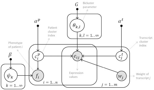
The probabilistic graphical model of SUBSTRA. The observed variables are shown with shaded circles and hyper-parameters are indicated by solid small circles. Other variables and parameters are shown with white circles. Please refer to the text for detailed explanation

The probabilistic graphical model of SUBSTRA is shown in Figure 1. All of the distributions and variables of this model are described in detail in Table 1. The central assumption is that the expression level of transcript j of patient i, which is indicated by e_ij, follows a probability distribution with parameter ${\theta }_{(c_i^p,c_j^e)}$ associated to bicluster $(c_i^p,c_j^t)$⁠. Depending on whether continuous or discrete expression data is considered, the probability distribution of variable e_ij can be Gaussian or categorical. We choose to use categorical expression data for two reasons: (i) using categorical data, modeled through a multi-nomial distribution, instead of continuous data, modeled through a Gaussian distribution, reduces the computational costs considerably due to simpler functional forms and parameters, and (ii) discrete expression data have been shown to improve the prediction accuracy and generality of the trained model (e.g. applicability to different array platforms) (Helman et al., 2004; Jung et al., 2015). We assume binary expression values where 0 indicates low and 1 indicates high expression levels. So, e_ij follows a Bernoulli distribution in SUBSTRA.

Table 1.

Variables and probabilistic relationships in the SUBSTRA model

Type	Name	Description	Distribution
Observed variables	eij	Expression status of transcript j of patient i	$e_{\mathit{ij}}\sim \mathit{Bernoulli}({\theta }_{c_i^p,c_j^t})$
	fi	Phenotype of patient i	$f_i\sim \mathit{Categorical}({\psi }_{c_i^p})$
	wj	Weight of transcript j	NA
Hyper-parameters	αp	Parameter of prior CRP for patient clusters	${\alpha }^p=1$
	αt	Parameter of prior CRP for transcript clusters	${\alpha }^t=1$
	G	Parameter for prior Beta base distribution of θ	G = 1
	β	Parameter for the prior Beta base distributions of ψ	Described in Section 2.3.1
Parameters	${\theta }_{k,l}$	Probability distribution of the values inside bicluster (k, l)	${\theta }_{k,l}\sim \mathit{Beta}(G)$
	ψk	Probability distribution of the values of the phenotypes of patient cluster k	${\psi }_k\sim \mathit{Dirichlet}(\beta )$
Latent variables	$c_i^p$	Cluster index for ith patient	$c_i^p\sim \mathit{CRP}({\alpha }^p)$
	$c_j^t$	Cluster index for jth transcript	$c_j^t\sim \mathit{CRP}({\alpha }^t)$

2.2 Feature weighting

In addition to the transcriptomic data, SUBSTRA incorporates the following information:

• Phenotype information: Phenotype of patient i shown by f_i. This information can be drug response, treatment effect, disease status, survival time, genetic risk score, etc.

• Transcript weights: A vector $w=[w_j]$ (⁠$1\le j\le m$⁠) of real values assigned to transcripts 1 to j. To compensate for the low influence of a single phenotype compared to the high dimensionality of the transcriptomic data, SUBSTRA propagates the effect of phenotype using phenotype-relevant transcript weights. Each weight is interpreted as the number of times that the corresponding transcript is considered during the biclustering. Thus, the higher the weight of a transcript, the stronger its effect on the biclustering. This variable is considered observed (shaded) in Figure 1, because, unlike the model latent variables that are inferred based on the joint probability of the model, we learn the transcript weights using a different objective function (i.e. prediction error) based on a Gradient Descent approach. More details are provided in Section 2.3.

As shown in Figure 1 and Table 1, phenotype of patient i indicated by f_i, follows a subtype-specific distribution with parameter ${\psi }_{c_i^p}$⁠. Furthermore, the transcript weights w_j influence the biclustering variables through expression variable e_ij. The information flow between the transcript weights and phenotypes are through e_ij and $c_i^p$ variables (this is possible because e_ij is observed and $c_i^p$ is latent). We use this information flow to adjust the transcript weights as described in Section 2.3. Without loss of generality, we assume that phenotype is a binary variable following a Bernoulli distribution in this paper. In practice, any distribution could be used based on the type of phenotype. A sample input for SUBSTRA and the expected output is shown in Figure 2.

Fig. 2.

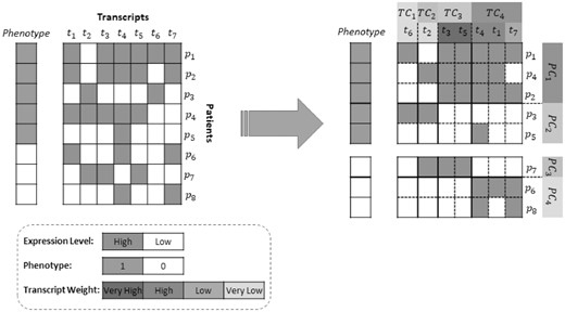
Input and output: The matrix on the left is reordered into the matrix on the right by SUBSTRA. The patients and transcripts are assigned to appropriate clusters and the transcript weights indicate the significance of features with regard to the phenotype. The patient and transcript clusters are formed in a way that the values inside biclusters are as consistent as possible, especially for those biclusters that are related to transcripts with higher weights. High-weight transcripts are those that form a biclustering more consistent with the phenotypes. For example, using the combination of transcripts in TC₃ and TC₄, one can produce the four patient clusters with homogeneous phenotypes (i.e. PC₁ to PC₄) as shown in the figure. So, the TC₃ and TC₄ transcripts are assigned high weights. On the other hand, t₂ and t₆ cannot form a consistent patient clustering when used alone or in combination with other transcripts and get low weights. Although in this sample the number of patient clusters is equal to the number of gene clusters, this is not a constraint in our algorithm

2.3 Parameter learning and inference

Parameter learning and inference are performed via Gibbs sampling.

The sampler infers the latent variables and learns the transcript weights simultaneously. The algorithm consists of three below phases.

2.3.1 Phase 0 (Initialization)

The latent variables of SUBSTRA (i.e. patient clusters $c_i^p$ and transcript clusters $c_j^t$⁠) are initialized randomly, such that two patients with different phenotypes are not assigned to the same cluster. This constraint satisfies the Assumption 3 stated in Section 1 during the initialization. However, the strictness of the constraint during the sampling can be controlled by the hyper-parameter β. If the mislabeling rate is low in the observed phenotypes, we should set the hyper-parameter β to a small value to make this constraint stricter. Otherwise, a larger β is used. The transcript weights are all initialized equal to μ, which is an input and indicates the magnitude of weights. If mu is large, the algorithm will be more sensitive to the values of transcript expressions and will fit faster to the data, increasing the probability of over-fitting or local optima. This works for the cases with strong relevant signals. On the other hand, when there are strong irrelevant signals in the data, a smaller μ is preferred as it provides more flexibility and increases the exploration space. We use cross-validation to tune this value. The value that produces more accurate phenotype prediction is selected, because higher accuracy implies more relevant biclustering and weighting.

2.3.2 Phase I

In this step, only the latent variables are sampled and the transcript weights are fixed. This is required since the initial random values of parameters can be misleading if used for adjusting the weights. In this phase, the Gibbs sampler uses the conditional probabilities of the latent variables. The conditional probabilities are computed based on the joint probability, which factorizes as below:

$$\begin{array}{c}P(e,w,f,c^p,c^t,\theta ,\psi |{\alpha }^p,{\alpha }^t,\beta ,G)\hfill \\ =P(c^p|{\alpha }^p)\times P(c^t|{\alpha }^t)\hfill \\ \times P(e|\theta ,c^p,c^t,w)P(\theta |G)\times P(f|\psi ,c^p)P(\psi |\beta )\end{array}$$

(1)

Considering this dependency structure and the distributions given in Table 1, the conditional probabilities of latent variables are computed as below:

$$\begin{array}{c}P(c_i^p=q|c_{-i}^p,e_{i.},w,f_i,c^t,\theta ,\psi ,{\alpha }^p)\hfill \\ \propto P(c_i^p=q|c_{-i}^p,{\alpha }^p)P(f_i|\psi ,c_i^p=q)P(e_{i.}|\theta ,c_i^p=q,c^t,w)\hfill \\ =\pi (q|c_{-i}^p,{\alpha }^p)\times {\psi }_q[f_i]\times \prod _{j=1}^m{({\theta }_{c_i^p,c_j^t}[e_{\mathit{ij}}])}^{w_j}\hfill \end{array}$$

(2)

$$\begin{array}{c}P(c_j^t=r|c_{-j}^t,e_{.j},w,c^p,\theta ,{\alpha }^t)\hfill \\ \propto P(c_j^t=r|c_{-j}^t,{\alpha }^t)P(e_{.j}|\theta ,c_j^t=r,c^p,w)\hfill \\ =\pi (r|c_{-j}^t,{\alpha }^t)\times \prod _{i=1}^n{\theta }_{c_i^p,c_j^t}[e_{\mathit{ij}}]\hfill \end{array}$$

(3)

where $\pi (q|c_{-i}^p,{\alpha }^p)$ is the CRP probability and is defined as below:

$$\pi (q|c_{-i}^p,{\alpha }^p)=\{\begin{array}{cc}\frac{{\alpha }^p}{n-1+{\alpha }^p}\hfill & \hspace{0.17em}\text{if}\hspace{0.17em}x\hspace{0.17em}\text{is}\hspace{0.17em}\text{an}\hspace{0.17em}\text{empty}\hspace{0.17em}\text{cluster}\hspace{0.17em}\\ \frac{\left|\right\{d|c_d^p=q\hspace{0.17em}\wedge \hspace{0.17em}d\ne i\}|}{n-1+{\alpha }^p}& \hspace{0.17em}\text{otherwise}\hspace{0.17em}\hfill \end{array}$$

(4)

m and n are respectively the numbers of transcripts and patients, ${\psi }_q[f_i]={\psi }_q$ if f_i = 1 and ${\psi }_q[f_i]=1-{\psi }_q$ if f_i = 0, and:

$${\theta }_{c_i^p,c_j^t}[e_{\mathit{ij}}]=\{\begin{array}{cc}{\theta }_{c_i^p,c_j^t}\hfill & \hspace{0.17em}\text{if}\hspace{0.17em}{e}_{\mathit{\text{ij}}}=1\\ 1-{\theta }_{c_i^p,c_j^t}& \hspace{0.17em}\text{otherwise}\hspace{0.17em}\end{array}$$

(5)

We use the predictive posterior distribution parameters to estimate the model parameters θ and ψ of equations 2 and 3 as follows:

$${\theta }_{q,r}=\frac{\text{no}.\hspace{0.17em}\hspace{0.17em}\text{of}\hspace{0.17em}\hspace{0.17em}1\prime \mathrm{s}\hspace{0.17em}\hspace{0.17em}\text{in}\hspace{0.17em}\hspace{0.17em}\text{bicluster}\hspace{0.17em}\hspace{0.17em}(\mathit{q},\mathit{r})+\mathrm{G}/2}{\text{no}.\hspace{0.17em}\hspace{0.17em}\text{of}\hspace{0.17em}\hspace{0.17em}\text{data}\hspace{0.17em}\hspace{0.17em}\text{points}\hspace{0.17em}\hspace{0.17em}\text{in}\hspace{0.17em}\text{bicluster}\hspace{0.17em}\hspace{0.17em}(\mathit{q},\mathit{r})+\mathrm{G}}$$

$${\psi }_q=\frac{\text{no}.\hspace{0.17em}\hspace{0.17em}\text{of}\hspace{0.17em}\hspace{0.17em}\text{patients}\hspace{0.17em}\hspace{0.17em}\text{in}\hspace{0.17em}\hspace{0.17em}\text{cluster}\hspace{0.17em}\hspace{0.17em}q \text{with} \text{phenotype} 1+\beta /2}{\text{no}.\hspace{0.17em}\hspace{0.17em}\text{of}\hspace{0.17em}\hspace{0.17em}\text{patients}\hspace{0.17em}\hspace{0.17em}\text{in}\hspace{0.17em}\hspace{0.17em}\text{cluster}\hspace{0.17em}\hspace{0.17em}q+\beta }$$

During Phase I, we repeat the following for each $c_i^p$⁠:

1. Estimate the parameters based on the current value of the model variables excluding $e_{i.}$⁠, f_i and $c_i^p$

2. Use equation 2 to sample $c_i^p$

Similarly for each $c_j^t$⁠, we:

1. Estimate the parameters based on the current value of the model variables excluding $e_{.j}$ and $c_j^t$

2. Use equation 3 to sample $c_j^t$

At each Gibbs sampling round we sample all latent variables as described above. As we use CRP, we consider the possibility of belonging to an empty cluster when sampling each latent variables for patients and transcripts. The sampling round is repeated until convergence or for a predefined number of iterations. The convergence is measured based on the Rand index similarity between the biclustering in two consecutive iterations, which is achieved when Rand index > 0.95 for patient and transcript clustering. Then we move to Phase II.

2.3.3 Phase II

In this phase, we adjust the transcript weights and simultaneously modify the biclustering structure. Since the weights should indicate the relevance of a transcript to the phenotype, we use the phenotype prediction error, which is a function of the weights, as the objective function for weight adjustment. The input to this phase is the latent variable values at the end of the previous phase. In addition to the steps in Phase I, we adjust transcript weights before sampling each $c_i^p$ in this phase following the below steps:

1. Estimate the parameters based on the current value of the model variables except $e_{i.}$⁠, f_i and $c_i^p$

2. Adjust the weights to reduce the phenotype prediction error for patient i

3. Use equation 2 to sample $c_i^p$

The weights are adjusted such that the objective function defined as the squared prediction error ${[1-p(f_i=x_i|\dots )]}^2$ (x_i is the true value of f_i) is minimized. Because the cluster assignment of patient i is unknown at this stage (i.e. we are about to sample it in step 3) and according to the information flow in the model (Fig. 1), we have:

$$\begin{array}{c}p(f_i=x_i|\dots )\hfill \\ =p(f_i=x_i|\psi ,e_{i.},c_{-i}^p,c^t,w,\theta ,{\alpha }^p)\hfill \\ =\sum _{q\in O}p(f_i=x_i,c_i^p=q|\psi ,e_{i.},c_{-i}^p,c^t,w,\theta ,{\alpha }^p)\hfill \\ =\sum _{q\in O}p(f_i=x_i|c_i^p=q,\psi )p(c_i^p=q|,c_{-i}^p,e_{i.},c^t,w,\theta ,{\alpha }^p)\hfill \\ \propto \sum _{q\in O}p(f_i=x_i|c_i^p=q,\psi )p(c_i^p=q,c_{-i}^p,e_{i.},c^t,w,\theta ,{\alpha }^p)\hfill \end{array}$$

(6)

where O is the set of occupied patient clusters. The second term in the last summation can be factorized based on the model (very similar to Equation 2). If we show the last summation above, which is a proportional value, by $\widehat{p}(f_i=x_i|\dots )$⁠, then we have:

$$p(f_i=x_i|\dots )=\frac{\widehat{p}(f_i=x_i|\dots )}{\sum _y\widehat{p}(f_i=y|\dots )}$$

(7)

where y indicates one of the values that the patient phenotype can take. Then the squared error of this probability value is used as the objective function. As in a Gradient Descent approach, we use the slope of this function to adjust the weights. So, the weights are updated as follows:

$$w_j=w_j+\nu \times 2\frac{\partial p(f_i=x_i|\dots )}{\partial w_j}[1-p(f_i=x_i|\dots )]$$

(8)

where ν is the learning rate and we set $\nu =\mu$⁠, the magnitude of weights, to maintain the magnitude of weights. The derivative term in the above equation is computed as below:

$$\frac{\partial p(f_i=x_i|\dots )}{\partial w_j}=\frac{\partial \frac{\widehat{p}(f_i=x_i|\dots )}{\sum _y\widehat{p}(f_i=y|\dots )}}{\partial w_j}$$

(9)

Let us define $p_y=\widehat{p}(f_i=y|\dots )$⁠. Then:

$$\frac{\partial p(f_i=y|\dots )}{\partial w_j}=\frac{\partial \frac{p_y}{\sum _y{p}_y}}{\partial w_j}=\frac{(\sum _y{p}_y)\frac{\partial p_y}{\partial w_j}-p_y\frac{\partial (\sum _y{p}_y)}{\partial w_j}}{{(\sum _y{p}_y)}^2}$$

(10)

So, we need to compute $\frac{\partial p_y}{\partial w_j}$ for every y. We have:

$$\begin{array}{c}\frac{\partial p_y}{\partial w_j}=\frac{\partial \sum _{q\in O}p(f_i=y|c_i^p=q,\psi )p(c_i^p=q,c_{-i}^p,e_{i.},c^t,w,\theta ,{\alpha }^p)}{\partial w_j}\hfill \\ =\sum _{q\in O}p(f_i=y|c_i^p=q,\psi )\times \partial \frac{p(c_i^p=q,c_{-i}^p,e_{i.},c^t,w,\theta ,{\alpha }^p)}{\partial w_j}\hfill \\ =\sum _{q\in O}{\psi }_q[y]\times \pi (q|c_{-i}^p,{\alpha }^p)\times \partial \frac{\prod _{l=1}^m{({\theta }_{q,c_l^t}[e_{\mathit{il}}])}^{w_l}}{\partial w_j}\hfill \\ =\sum _{q\in O}{\psi }_q[y]\times \frac{\left|\right\{d|c_d^p=q\hspace{0.17em}\wedge \hspace{0.17em}d\ne i\}|}{n-1+{\alpha }^p}\hfill \\ \times \text{log}({\theta }_{q,c_j^t})\hspace{0.17em}\prod _{l=1}^m{({\theta }_{q,c_l^t}[e_{\mathit{il}}])}^{w_l}\hfill \end{array}$$

(11)

Computing the left-hand-side of Equation 10 based on the Equation 11 and then using it in Equation 8 for computing the new weights is straight-forward. The new weights are accepted only if they reduce the squared error. Otherwise, the algorithm continues with the previous weights and goes to the next patient.

In this phase, a certain number of iterations is executed and the model performance in terms of the Area Under the Receiver Operating Characteristic Curve (AUC) over the training set is monitored. Finally, the model that corresponds to the iteration with the highest AUC is selected. Ties are broken with respect to the Mean Squared Error (MSE) of the predicted probabilities. Although the training set AUC and MSE are used for model selection, over-fitting is avoided because the data corresponding to patient i is not included in updating the weights for that patient.

3 Experiments and results

In this section we describe the experiments performed for testing the accuracy of SUBSTRA. The method produces two types of outputs: predictive outputs (predicted phenotypes) and descriptive outputs (i.e. patient strata, transcript clusters and transcript weights). We benchmark against other methods with respect to these outputs.

3.1 Predictive performance evaluation

To investigate the predictive ability of SUBSTRA, it is benchmarked against the following methods:

• Support Vector Machine (SVM): A well-known state-of-the-art prediction method with high accuracy. The implementation of SVM in R package ‘e1071’ is used.

• Regularized Logistic Regression (LR): A popular prediction method that assigns model-based (not ad-hoc) weights to the predictor features. We used the Elastic Net Generalized Linear Models implementation in R package ‘caret’.

• Predictive Chain (PCH): This method is evaluated as a simple baseline method that performs biclustering and prediction in two separate steps, rather than in one integrated step as SUBSTRA does. It first applies NMF (Lee and Seung, 1999) (a popular biclustering method) for deriving a low-rank representation of the patients and then trains the LR model on that representation. We investigate whether using NMF output will have positive or negative effects on the prediction accuracy of LR.

The Area Under the Receiver Operating Characterisitics (AUC) metric is computed to measure the prediction accuracy of all three methods through nested CV and with several executions to accommodate for random initialization (see Supplementary Section C for more details).

3.2 Descriptive performance evaluation

We benchmarked the biclustering accuracy of SUBSTRA against similar biclustering methods that do not consider phenotype data (i.e. unsupervised patient stratification). SUBSTRA performs exhaustive and exclusive biclustering with constant values inside the biclusters. Based on a review over 47 biclustering algorithms for gene expression data provided by Pontes et al. (2015), we found HARP (Yip et al., 2004) to be the most consistent method with these features. Two other comparable methods not listed in Pontes et al. (2015), include B2PS (Khakabimamaghani and Ester, 2016), which is an exhaustive, exclusive and constant value biclustering method, and NMF.

As stated in Section 1, many existing supervised stratification methods either leverage several phenotypes or make specific assumptions for compound phenotypes, e.g. assume survival data. This makes it hard to compare SUBSTRA with those methods. Therefore, we define an additional simple baseline method that first identifies feature weights using LR. Then, the feature weights are given to weighted NMF (wNMF) (Wang et al., 2006) for biclustering. We call this method Descriptive Chain (DCH). This is to investigate the influence of the provided weights on the biclustering accuracy, as well as comparison against SUBSTRA’s biclustering.

We compare SUBSTRA against HARP, B2PS, NMF and DCH in terms of the following metrics:

• Patient Strata: Whenever the ground-truth patient clusters are available, we use Rand index to measure the patient clustering accuracy.

• Transcript Clustering: Transcripts fall into two categories of relevant (signal) and irrelevant (noise) to the phenotype. We only focus on the clustering results for the relevant transcripts. Two metrics, cluster purity and class purity are used for evaluation. Clusters refer to the outputs of the methods and classes refer to the ground-truth transcript clusters. Class purity (CSP) measures how well the true signal clusters are separated from each other by the method. Cluster purity (CLP) indicates how much of the signal transcripts are captured in the method clusters. Together, these two metrics reflect how well the method has been able to capture the true signal clusters. More details are provided in Supplementary Section D. For HARP, we note that it is only exclusive with regard to patient clustering and might produce overlapping transcript clusters. Thus, only CLP can be reported for this method.

• Transcript Weights: Pearson correlation coefficient between the ground-truth weights and method weights are reported when the ground-truth information is available. When unavailable, GO term enrichment analysis of the top ranked genes is used as described later.

3.3 Experiments with synthetic data

We used synthetic data to have access to the ground-truth information to benchmark SUBSTRA for detecting the true patient and transcript clusters, true feature weights and accurate prediction. Different synthetic datasets were generated considering the assumptions mentioned in Section 1. In separate simulations, we tested different types of relations between the transcript clusters and the phenotype: AND, OR and XOR. For this purpose, we assumed that the expression values of two transcript clusters A and B are correlated with the phenotype through the mentioned relations. As an example, for an XOR relationship, the value of phenotype will be 1 if and only if the transcripts of only one of the clusters A or B are expressed.

Each dataset consists of 200 patients constituting 4 patient clusters with four different possible combinations of parameters for signals A and B (i.e. A high-B high, A high-B low, A low-B high and A low-B low). Each of these two clusters includes 10 transcripts. Bicluster parameters larger than 0.5 indicate high expression and vice versa. A third transcript cluster is included as the noise, with parameter equal to 0.5 across different patient clusters (i.e. biclusters with Bernoulli distribution with parameter 0.5). The values of parameters for different settings are provided in Supplementary Section A. The performance of the three methods are compared for different datasets with 90, 95 or 99% of transcripts belonging to the noise cluster. These datasets will respectively contain 200, 400 and 2000 transcripts 20 of which are relevant signals and the rest are noise.

To avoid biases towards our own assumptions, we include another synthetic microarray dataset introduced in Abu-Jamous et al. (2015). This dataset, to which we refer as UNCLES (the title of the paper), consists of two patient classes (positive and negative) and three gene clusters. The gene cluster C1 (75 genes) includes genes consistently co-expressed for all patients, and the gene cluster C2 (85 genes) includes genes consistently co-expressed only in the positive class while being poorly co-expressed in the negative class. Among the two clusters, C1 is more correlated with the patient classes as it has in general higher expression in the positive class and lower expression in the negative class. Accordingly, although we evaluate the methods for detecting the two clusters, we only consider C1 when evaluating the capabilities of the methods in up-weighting the phenotype-relevant genes. The rest of the genes (1040 genes) are poorly co-expressed everywhere and are considered noise. The dataset contains 42 positive and 40 negative patients. The UNCLES dataset contains continuous data. We use the original continuous as well as the discretized data. To monitor the sensitivity to different discretization methods, three different approaches, namely Equal-Frequency Binning (EFB), Equal-Width Binning (EWB) and k-means (KM), are used for discretization as described in Jung et al. (2015).

Table 2 shows the predictive and descriptive results for different simulation settings. Among the methods, HARP and NMF has the lowest performance for most of the datasets with respect to patient stratification. Adding supervision to NMF as in DCH improves the results in high noise datasets (i.e. AND and OR 99%), however, it does not have significant effects on the other cases. B2PS and SUBSTRA perform relatively better than other methods both in our simulations and UNCLES dataset. SUBSTRA outperforms B2PS considerably (difference larger than 0.05) in high noise datasets as well as XOR relationship, which is more complex than AND and OR.

Table 2.

Results for the experiments with the synthetic data

Metric	Type	Method	AND			OR			XOR			UNCLES
			90%	95%	99%	90%	95%	99%	90%	95%	99%	EFB	EWB	KM	NO
PC Rand,#	Descriptive	HARP	0.66, 4	0.63, 4	0.61, 4	0.66, 4	0.63, 4	0.63, 4	0.66, 4	0.66, 4	0.61, 4	0.78, 6	0.72, 6	0.74, 6	0.68, 6
		B2PS	0.91, 8	0.91, 10	0.41, 8	0.87, 8	0.89, 10	0.89, 9	0.84, 8	0.87, 9	0.85, 10	0.86, 19	0.86, 19	0.86, 18	NA
		NMF	0.68, 4	0.67, 4	0.62, 4	0.70, 4	0.69, 4	0.62, 4	0.71, 4	0.70, 4	0.62, 4	0.82, 8	0.77, 6	0.80, 7	0.79, 9
		DCH	0.70, 4	0.69, 4	0.70, 4	0.71, 4	0.71, 4	0.75, 4	0.69, 4	0.62, 4	0.61, 4	0.80, 8	0.75, 6	0.77, 7	0.74, 9
		SUBSTRA	0.96, 10	0.93, 8	0.89, 12	0.87, 12	0.92, 10	0.95, 11	0.95, 10	0.96, 9	0.94, 11	0.85, 15	0.82, 9	0.82, 10	NA
CSP%, CLP%	Descriptive	HARP	NA, 25	NA, 07	NA, 01	NA, 24	NA, 09	NA, 02	NA, 27	NA, 14	NA, 03	NA, 15	NA, 23	NA, 35	NA, 13
		B2PS	100, 100	95, 100	65, 02	100, 100	100, 100	100, 100	100, 100	100, 100	100, 100	83, 95	81, 96	93, 97	NA
		NMF	100, 30	100, 11	75, 02	100, 24	100, 12	95, 02	100, 27	100, 14	90, 02	97, 21	94, 26	81, 28	66, 32
		DCH	90, 60	85, 89	85, 01	80, 55	50, 05	65, 15	80, 21	70, 12	95, 01	81, 10	78, 29	97, 26	94, 26
		SUBSTRA	100, 100	100, 100	100, 100	100, 100	100, 100	100, 100	100, 100	100, 100	100, 100	98, 97	79, 97	89, 97	NA
WPC	Descr.	DCH (LR)	0.58*	0.68*	0.59*	0.30*	0.33*	0.31*	0.10	0.04	−0.01	−0.01	0.08	0.03	−0.04
		SUBSTRA	0.65*	0.72*	0.70*	0.59*	0.54*	0.47*	0.49*	0.44*	0.28*	0.21*	−0.05	0.14*	NA
AUC	Predictive	LR	0.88	0.84	0.85	0.72	0.73	0.58	0.46	0.52	0.60	0.74	0.51	0.56	0.99
		SVM	0.87	0.82	0.70	0.65	0.61	0.55	0.62	0.62	0.34	0.98	0.94	0.94	0.88
		PCH	0.78	0.71	0.53	0.78	0.68	0.63	0.44	0.44	0.40	0.94	0.51	0.55	0.81
		SUBSTRA	0.97	0.97	0.97	0.91	87	0.93	0.91	0.89	0.88	1.00	0.96	0.97	NA

Note: Abbreviations used include PC Rand,#—Rand index for patient clustering (comparison with the ground truth) and the number of patient clusters, CSP%, CLP%—class purity and cluster purity (described in Section 3.2) as percentage, WPC—Pearson correlation coefficient between the true weights and the method’s weights with statistically significant results (after Bonferroni correction) marked by *, and NO—no discretization. Best performance in each dataset is shown in bold if the gap with the second best performance is larger than or equal to 0.05 for Rand index, purity and AUC and larger than or equal to 0.1 for WPC when at least one of the correlations is significant.

With respect to transcript clustering, HARP and NMF has similarly lower CLP in most of the cases. The reason is that both methods detect uniformly large and impure clusters. On the other hand, NMF has superior ability in separating the signal clusters from each other compared to DCH. Although, adding supervision in DCH improves cluster purity (CLP) for some low-noise datasets compared to solo NMF, it increases the chance of mixing the true signal clusters in a single transcript cluster (lower CSP). Top methods with respect to transcript clustering are B2PS and SUBSTRA, with SUBSTRA being superior in certain cases (high noise AND and EFB UNCLES). This indicates that supervision as in SUBSTRA improves the clustering quality.

Table 2, also, shows the transcript weighting results for SUBSTRA and DCH. The values indicate the correlation between the method and the ground-truth weights. The ground-truth weights are produced by assigning weight 1 to the signal transcripts (members of A, B and C1 clusters) and 0 to the other transcripts. Based on the results, SUBSTRA produces consistently more correlated weights for the synthetic data than DCH, which uses LR for weighting. This can be associated to the probabilistic nature of the method and its ability to capture more complex relationships like XOR, which are not detectable by linear methods such as LR (note the low correlation values of DCH for XOR and UNCLES). Transcript clustering in SUBSTRA can increase the weight consistency inside the transcript clusters beside improving the accuracy of the weights due to inter-cluster discrepancies. The descriptive results are visualized in Supplementary Section A.

Regarding the AUC measures in Table 2, SUBSTRA, also, outperforms the other predictive benchmark methods in most of the experiments and is more robust to the noise levels and the task complexity. On the other hand, PCH and LR are sensitive to noise and the type of discretization and SVM is sensitive to noise but robust to the discretization method. Binary data, compared to continuous data, is associated with better performance except for the predictive accuracy of LR.

3.4 Experiments with real data

We also tested SUBSTRA with real data. These datasets are listed in Table 3. The Kidney 1 and 2 datasets are taken from studies Khatri et al. (2013) and Einecke et al. (2010). They include baseline gene expression profiles for patients before kidney transplantation and whether the patient rejected the transplantation (phenotype). We also used a dataset from the Cancer Cell Line Encyclopedia (CCLE) (Barretina et al., 2012), which provides a collection of genomic information (including baseline transcriptomic data) and pharmacological profiles (including response to various drugs for several cell lines derived from different tissues). A subset of cell lines which had information about their response to AZD6244 (a drug that targets MEK) was selected from this dataset. Response to the drug was recorded in terms of IC50. We used a cut-off value of 7 to discretize IC50 values to 0 (not responding) and 1 (responding). Two datasets, namely Lung Cancer from Gordon et al. (2002) and Multiple Myeloma from Tian et al. (2003), were also used from the R package ‘datamicroarray’ (Ramey, 2011). The package is a collection of microarray datasets with phenotypes. They are from different studies and can be used for machine learning.

Table 3.

Datasets used in the predictive and descriptive experiments

Dataset	#Patients	#Features	Phenotype	Neg.-Pos.	Reference
Kidney 1	282	18, 089	Kidney transplant response	63–37%	Einecke et al. (2010)
Kidney 2	101	18, 988	Kidney transplant response	57–43%	Khatri et al. (2013)
Drug Response	490	42, 869	Response to AZD6244	26–74%	Barretina et al. (2012)
Multiple Myeloma	173	12, 625	Existence of focal bone lesions	21–79%	Tian et al. (2003)
Lung Cancer	181	12, 533	Malignant Pleural Mesothelioma (MPM) or Adenocarcinoma (ADCA) of the Lung	17% (MPM)- 83% (ADCA)	Gordon et al. (2002)

All datasets are pre-processed. For each dataset, the first 5000 features with the highest coefficient of variation are selected. Then, the three mentioned discretization methods are used to binarize the continuous expression data into 0 (low) and 1 (high). These methods are non-parametric and does not depend on any threshold. Continuous data is also considered where applicable.

Since no ground-truth data are available about patient strata and transcript clusters, we only benchmarked the predictive performance and transcript weights of SUBSTRA against the comparison partners. All methods were executed on the same cross-validation folds and experiments were repeated and averaged to accommodate for the random initialization effects. More details are provided in Supplementary Section C.

Figure 3 shows the predictive results for the above datasets. According to these results, all methods have in general similar predictive performance when considering the best performing configuration (i.e. discretization). Looking closer LR has a slightly better performance than the others in three out of five experiments. SUBSTRA and SVM are performing similar taking all experiments into account. SUBSTRA produces more stable results than the other methods as reflected in the error bars. Considering similar discretizations, SUBSTRA performs better than the predictive alternative PCH. Using continuous data, which is not yet implemented in SUBSTRA, PCH approaches SUBSTRA, especially in ‘Multiple Myeloma’ and ‘Drug Response’ datasets. These results match those of simulation experiments and indicate that simple chaining of the existing methods does not reproduce the quality of SUBSTRA. As a multi-purpose method, SUBSTRA, provides reasonable predictive performance while producing more relevant descriptive outputs (as described later), thus maintaining a good trade-off between accuracy and interpretability that is lacking in most of the existing methods.

Fig. 3.

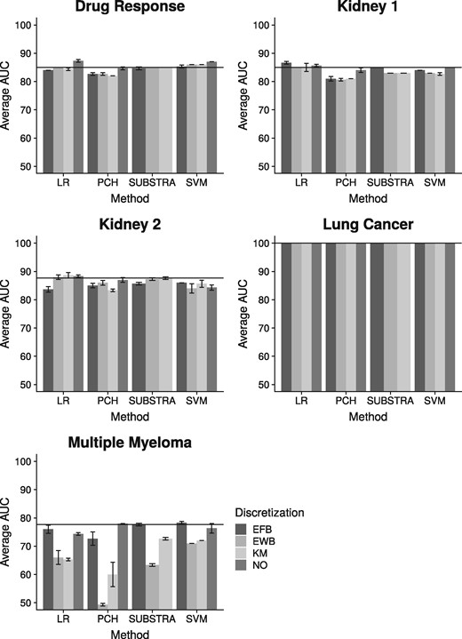
Predictive results for the real data: The horizontal line indicates the best performance of SUBSTRA. The error bars are based on standard deviation. NO—no discretization

Discretization has positive effect for some datasets and methods and negative effects for the others. However, there is a general indifference with respect to the discretization techniques. The exception here is ‘Multiple Myeloma’, for which EFB resulted in better performance than the other techniques, matching the findings in Jung et al. (2015).

To evaluate the plausibility of the weights assigned to the transcripts, we compared SUBSTRA with DCH using the following analysis. We ran both methods using the pre-processed data corresponding to the best predictive performance (among EFB, EWB and KM) in Figure 3. Experimental settings are described in Supplementary Section C. Then, the transcripts were sorted in descending order with respect to the weights obtained by each method. Top 100 transcripts were selected for each dataset and each method. We mapped transcripts to genes, and conducted Gene Ontology (GO) enrichment analysis for the top 100 genes for each dataset. The only exception was the ‘Kidney 1’ dataset for which we selected top 200 to obtain enriched GO terms for at least one of the methods (top 100 genes were not significantly associated to any GO term). To compare consistency of the top genes across the two methods, we computed the GO terms that are significantly enriched with top genes (q-value < 0.05) for both methods (i.e. common enriched GO terms). Then, we compared the q-values associated to these GO terms by the two methods to see which method produces more significant enrichment for the common terms. We used paired Wilcoxon signed-rank test on the logarithms of the q-values. Next, we performed a similar analysis for the top transcript cluster of each method according to the average weight. For ‘Drug Response’, since the top 3 clusters of none of the methods were significantly associated with any GO terms, we looked at the 4th clusters.

The statistical significance of the difference between the enrichment of the top genes and clusters selected by the two methods are shown in Table 4. According to these results, top genes of SUBSTRA for ‘Lung Cancer’ and ‘Kidney 2’ result in significantly stronger enrichment. For ‘Kidney 1’, DCH top genes were not associated with any GO terms while SUBSTRA top genes were related to 15 significantly enriched GO terms indicative of higher consistency among them. For ‘Multiple Myeloma’ and ‘Drug Response’, there was no statistically significant difference the two methods. Overall, SUBSTRA detected significantly more relevant genes in two out of five experiments and was equally well in the others, which indicated its descriptive abilities compared to existing methods.

Table 4.

Comparison between the weights assigned by SUBSTRA and DCH to the transcripts

	Metric	Kidney 1	Kidney 2	Drug Response	Multiple Myeloma	Lung Cancer
Genes	WSRT(Com.)	NA(0)	0.03(6)	0.65(9)	0.87(67)	0.01(36)
	SUBSTRA	NA	−20.96	−4.20	−6.34	−4.86
	DCH	NA	−5.33	−4.41	−6.03	−6.04
Cluster	WSRT(Com.)	0.00(69)	NA(0)	NA(0)	NA(0)	NA(0)
	SUBSTRA	−31.53	NA	NA	NA	NA
	DCH	−4.34	NA	NA	NA	NA

Note: Abbreviations used include WSRT(Com.)—Wilcoxon Signed-Rank Test (WSRT) P-value and the number of common GO terms in the parentheses. The top and bottom halves of the table correspond respectively to the evaluation of the top weighted genes and cluster. In each of the two parts, the second and third rows show the mean of the logarithm of the q-values of the enrichment tests for SUBSTRA and DCH, respectively. NAs indicate the situations when there have been no common enriched GO term between the two methods. In all NA cases, this was due to one of the methods (DCH) having empty enriched GO term set. The best performances are shown in bold.

For the top transcript clusters, the results were more different among the two methods. In four out of five cases, no enrichment was detected for DCH while SUBSTRA could detect significantly enriched clusters. The reason might be the relatively small clusters that wNMF detected. For ‘Kidney 1’, both methods produced large top clusters, but SUBSTRA’s cluster was very significantly more enriched. This indicates the meaningfulness of the transcript clusters detected by SUBSTRA. In the next section, we look at the relevance of these clusters to the phenotypes.

3.5 SUBSTRA finds relevant transcript clusters

SUBSTRA detects transcript clusters that define patient subtypes. Sorting clusters by the average of the transcript weights gives an indication of their relevance to the phenotype under consideration. We further analyzed the top 5 transcript clusters that SUBSTRA identified for each real dataset through Gene Ontology (GO) and Pathway (PW) enrichment analysis. The results indicate the uniform relevance of the identified transcript clusters and match the existing literature beside detecting novel signals requiring further investigation. The detailed procedures and results are provided in Supplementary Section B. In the following paragraphs we provide the highlights of the descriptive results based on the gene clusters identified in SUBSTRA’s output.

The ‘Kidney 1’ dataset was obtained from biopsies extracted more than a year after the kidney transplants (Einecke et al., 2010). The authors of this study developed a classifier for transplant failure versus acceptance, and identified 886 genes whose expression was significantly associated with graft failure. Of the 30 top genes most frequently used by the classifier, five (HAVCR1, ITGB3, LTF, PLK2 and SERPINA3) were clustered in the second top cluster (C2) identified by SUBSTRA. SUBSTRA clusters suggests that inflammatory processes (cluster C1) can be implicated separately from pathways associated with cellular death and differentiation, extra-cellular matrix organization and circulatory system development (cluster C2), in allograft rejection. In fact Einecke et al. (2010) implicate inflammatory processes in early graft rejection, and pathways enriched in SUBSTRA cluster C2 in later graft loss, suggesting that SUBSTRA correctly captures and distinguished among different mechanisms responsible for rejection (see Supplementary Figs SB2 and SB3). Although genes in C3, a cluster enriched in transmembrane transport, and C5, a cluster enriched in organ morphogenesis and tissue development, are present among the 886 classifying genes in the original publication, SUBSTRA makes a novel prediction that these additional mechanisms play distinct and central roles in graft rejection.

In the study associated with the ‘Kidney 2’ dataset, Khatri et al. (2013) identified a ‘common rejection module’ consisting of 11 genes that were differentially expressed in rejection of transplanted organs: BASP1, CD6, CD7, CXCL9, CXCL10, INPP5D, ISG20, LCK, NKG7, PSMB9, RUNX3 and TAP1. SUBSTRA placed six of these genes—CXCL9, CXCL10, LCK, NKG7, PSMB9 and RUNX3, in the fourth gene cluster, supporting the conclusions of Khatri et al., that these genes form a distinct module that differentiates graft rejection from non-rejection. The second top cluster shows enrichment of ‘graft versus host disease’, allograft rejection, immune signaling pathways, as well as related pathways such as cell, leukocyte and lymphocyte activation (see Supplementary Figs SB5 and SB6). The remaining gene clusters (except C3) exhibit similar enrichment of immune response pathways.

‘Drug Response’ dataset (Barretina et al., 2012) contains gene expression information from cancer cell lines treated with AZD6244, known as selumetinib. Selumetinib’s target, MEK, is implicated in the epithelial-mesenchymal transition (EMT), which is an important step in the initiation of metastasis (Bartholomeusz et al., 2015). Among many other physiological changes, EMT involves the loss of cell-cell junctions such as tight junctions that are characteristic of epithelial cells. Our method identifies a transcript cluster related to EMT involved in cell–substrate adhesion as key pathways that respond to selumetinib (see Supplementary Fig. SB8).

In ‘Multiple Myeloma’, Tian et al. (2003) identified DKK1 as an important gene involved in the formation of focal bone lesions. As an inhibitor of the Wnt signaling pathway, DKK1’s exact role in modulating this phenotype can be related to any of the pathway’s many downstream effects, such as cell fate determination, cell motility, body axis formation, cell proliferation and stem cell renewal (Komiya and Habas, 2008). SUBSTRA recapitulated the original analysis by assigning the greatest weight to DKK1 within the third relevant cluster. Interestingly, this cluster also harbors some of the most significantly enriched pathways. Gene set enrichment analysis identified the cell cycle and MAPK, signaling as pathways enriched in genes of this cluster (C3 in Supplementary Figs SB10 and SB11). This result suggests that DKK1 might be modulating cell proliferation as opposed to other cellular processes associated with the Wnt signaling pathway. Furthermore, previous work has shown an interplay between the Wnt and MAPK signaling pathways in skeletal development (Zhang et al., 2014). MAPK, signaling may be playing an important role in the formation of osteolytic lesions, a potential discovery that is not described in the original study. This shows that SUBSTRA biclustering and weight assignment can complement other methods such as differential gene expression analysis to provide additional biological context.

For the ‘Lung Cancer’ dataset, Gordon et al. (2002) originally identified eight genes differentially expressed between adenocarcinoma of the lung (ADCA) and malignant pleural mesothelioma (MPM): CALB2, ANXA8, EPCAM, CLDN7, NKX2-1, CD200, PTGIS and COBLL1. SUBSTRA reported all but one gene (CLDN7) in the top 3 transcript clusters, although other claudin genes, namely CLDN3 and CLDN4, were included in the top cluster. Consistent with the eight genes, cell and focal adhesion are among the enriched GO terms and KEGG pathways in the top 5 transcript clusters (see Supplementary Figs SB13 and SB14). Moreover, SUBSTRA suggests several additional pathways, including extracellular receptor interaction, MAPK signaling and cytokine receptor interactions, that may biologically distinguish ADCA and MPM.

3.6 Runtime of SUBSTRA

In a series of experiments on synthetic data (see Supplementary Section E), the influence of the input size factors on the runtime of SUBSTRA were identified. The studied factors included the number of patients n, the number of transcripts m, the number of patient strata and the number of transcript clusters. The runtime was scaled linearly with respect to the first three factors, however, the last factor did not have any correlation with the runtime in our experiments.

4 Conclusion

In this paper, an integrative Bayesian probabilistic model for simultaneous analysis of transcriptomic and phenotype data is presented. The model, called SUBSTRA, learns patient strata relevant to a phenotype and detects corresponding transcript clusters. The method also assigns weights to the transcripts based on their relevance to the phenotype and allows for interpretable prediction. SUBSTRA achieves both good interpretability (i.e. produces meaningful patient clusters, transcript clusters and transcript weights) and accurate phenotype prediction, which is lacking in the state-of-the-art methods for phenotype prediction (Valdes et al., 2016) such as SVM.

Based on the simulation results, the combination of transcriptomic and phenotype data improves patient stratification results and helps detecting relevant linear and non-linear signals in situations with high noise levels. The biclustering also improves the prediction accuracy in certain simulation experiments. We carried out gene set enrichment analysis of the transcripts identified as important by SUBSTRA in relevant biological scenarios, such as kidney rejection and drug response. We found that SUBSTRA selects more consistent genes with better enrichment values compared to regularized logistic regression models in most of the experiments. Also, analyzing the transcript clusters detected by SUBSTRA indicates that they capture key biological mechanisms that drive the differential fates of these samples and shed light on factors driving predictive performance. These clusters are shown to be more consistent than the alternative methods discussed in the paper and the prediction accuracy of SUBSTRA is shown to be comparable with the common single-purpose predictive methods, such as LR and SVM.

We employ Gibbs sampling in SUBSTRA as the inference method. One direction for future work can be using more efficient approaches like variational inference or parallelizing the inference. As another future work, we plan to extend SUBSTRA to incorporate continuous expression data and more patient and transcript information, such as pathways and interaction data. This might further improve the performance as well as the general applicability of SUBSTRA to a wide range of diseases and conditions. In scenarios with temporary data access contracts, only the model learned from data is available, but not the dataset itself. For such scenarios, we plan to explore methods for Lifelong Machine Learning using SUBSTRA based on the Bayesian properties of the model. The Bayesian nature of this method allows for incorporation of prior knowledge extracted from previously available datasets when training a new model, which might compensate for the lack of access to those data.

Conflict of Interest: none declared.

Author notes

The authors wish it to be known that, in their opinion, Martin Ester and Daniel Ziemek authors should be regarded as Joint last Authors.