Rapid alignment-free phylogenetic identification of metagenomic sequences

Abstract

Motivation

Taxonomic classification is at the core of environmental DNA analysis. When a phylogenetic tree can be built as a prior hypothesis to such classification, phylogenetic placement (PP) provides the most informative type of classification because each query sequence is assigned to its putative origin in the tree. This is useful whenever precision is sought (e.g. in diagnostics). However, likelihood-based PP algorithms struggle to scale with the ever-increasing throughput of DNA sequencing.

Results

We have developed RAPPAS (Rapid Alignment-free Phylogenetic Placement via Ancestral Sequences) which uses an alignment-free approach, removing the hurdle of query sequence alignment as a preliminary step to PP. Our approach relies on the precomputation of a database of k-mers that may be present with non-negligible probability in relatives of the reference sequences. The placement is performed by inspecting the stored phylogenetic origins of the k-mers in the query, and their probabilities. The database can be reused for the analysis of several different metagenomes. Experiments show that the first implementation of RAPPAS is already faster than competing likelihood-based PP algorithms, while keeping similar accuracy for short reads. RAPPAS scales PP for the era of routine metagenomic diagnostics.

Availability and implementation

Program and sources freely available for download at https://github.com/blinard-BIOINFO/RAPPAS.

Supplementary information

Supplementary data are available at Bioinformatics online.

1 Introduction

Inexpensive high-throughput sequencing has become a standard approach to inspect the biological content of a sample. Well-known examples range from health care, where sequencing-based diagnostics are being implemented in many hospitals and in reaction to disease outbreaks (Gardy and Loman, 2017; Gilchrist et al., 2015), to environmental and agricultural applications, where the diversity of the microorganisms in soil, water, plants, or other samples can be used to monitor an ecosystem (Deiner et al., 2017; Porter and Hajibabaei, 2018). Furthermore, with the advent of sequencing miniaturization, the study of environmental DNA will soon be pushed to many layers of society (Gilbert, 2017; Zaaijer et al., 2016).

Metagenomics is the study of the genetic material recovered from this vast variety of samples. Contrary to genomic approaches studying a single genome, metagenomes are generally built from bulk DNA extractions representing complex biological communities that include known and yet unknown species (e.g. protists, bacteria, viruses). Because of the unexplored and diverse origin of the DNA recovered, and because of the sheer volume of sequence data, the bioinformatic analysis of metagenomes is very challenging. Metagenomic sequences are often anonymous, and identifying a posteriori the species from which they originated remains an important bottleneck for analyses based on environmental DNA.

Several classes of approaches are possible for taxonomic classification of metagenomic sequences, the choice of which will generally depend on the availability of prior knowledge (e.g. a reference database of known sequences and their relationships) and a tradeoff between speed and precision. For instance, without prior knowledge, the exploration of relatively unknown clades can rely on unsupervised clustering (Mahé et al., 2014; Ondov et al., 2016; Sedlar et al., 2017). The precision of this approach is limited, and clusters are generally assigned to taxonomic levels via posterior analyses involving local alignment searches against reference databases. An alternative is to contextualize local alignments with taxonomic metadata. For instance, MEGAN (Huson et al., 2007, 2016) assigns a query metagenomic sequence (QS for simplicity) to the last common ancestor (LCA) of all sequences to which it could be aligned with a statistically significant similarity score (e.g. using BLAST or other similarity search tools). A faster alternative is to build a database of taxonomically informed k-mers which are extracted from a set of reference sequences. Classification algorithms then assign a QS to the taxonomic group sharing the highest number of k-mers with the QS (Ames et al., 2013; Liu et al., 2018; Müller et al., 2017; Wood and Salzberg, 2014). All of these approaches use simple sequence similarity metrics and no probabilistic modeling of the evolutionary phenomena linking QSs to reference sequences. The advantage is that, particularly in the case of k-mer-based approaches, these methods facilitate the analysis of millions of QSs in a timescale compatible with large-scale monitoring and everyday diagnostics.

Nevertheless, in many cases a precise identification of the evolutionary origin of the QSs is desired. This is particularly true for medical diagnostics where adapted treatments will be administered only after precise identification of a pathogen (Butel, 2014; Trémeaux et al., 2016). In the case of viruses (under studied and characterized by rapid evolution), advanced evolutionary modeling is necessary to perform detailed classifications. A possible answer in this direction may be the use of phylogenetic inference methods. However, the standard tools for phylogenetic inference are not applicable to metagenomic datasets, simply because the sheer number of sequences cannot be handled by current implementations (Izquierdo-Carrasco et al., 2011).

A solution to this bottleneck is phylogenetic placement (PP) (Berger et al., 2011; Matsen et al., 2010). The central idea is to ignore the evolutionary relationships between the QSs and to focus only on elucidating the relationships between a QS and the known reference sequences. A number of reference genomes (or genetic markers) are aligned and a ‘reference’ phylogenetic tree is inferred from the resulting alignment. This reference tree is the backbone onto which the QSs matching the reference genomes will be ‘placed’, i.e. assigned to specific edges. When a QS is placed on an edge, this is interpreted as the evolutionary point where it diverged from the phylogeny. Note that when the placement edge of a QS is not incident to a leaf of the tree, the interpretation is that it does not belong to any reference genome, but to a yet unknown/unsampled genome for which the divergence point has been identified. This is different from LCA-based approaches where a QS assigned to an internal node usually means that it cannot be confidently assigned to any leaf of the corresponding subtree. Currently, only two PP software implementations are available: PPlacer (Matsen et al., 2010; McCoy and Matsen, 2013) and EPA (until recently a component of RAxML) (Berger et al., 2011). They are both likelihood-based, i.e. they try to place each QS in the position that maximizes the likelihood of the tree that results from the addition of the QS at that position. Alternative algorithms were also described, but implementations were not publicly released (Brown and Truszkowski, 2013; Filipski et al., 2015). These methods have some limitations: (i) likelihood-based methods require an alignment of each QS to the reference genomes prior to the placement itself, a complex step that may dominate the computation time for long references, and (ii) despite being much faster than a full phylogenetic reconstruction, they struggle to scale with increasing sequencing throughputs. Recently, the development of EPA-ng (Barbera et al., 2019) provided an answer to the second point via the choice of advanced optimization and efficient parallel computing. But no fundamental algorithmic changes were introduced, and the method still relies on a preliminary alignment.

To avoid these bottlenecks, we have developed the PP program RAPPAS (Rapid Alignment-free Phylogenetic Placement via Ancestral Sequences). The novelty of our approach rests on two key ideas: (i) a database of phylogenetically informed k-mers (‘phylo-kmers’) is built from the reference tree and reference alignment, (ii) QSs are then placed on the tree by matching their k-mers against the database of phylo-kmers. For a specific group of organisms, the maintenance of the RAPPAS database can be seen as a periodic ‘build-and-update’ cycle, while the PP of new metagenomes becomes a scalable, alignment-free process compatible with day-to-day routine diagnostics. This algorithmic evolution bypasses the alignment of QSs to the reference required by existing algorithms. For short reads RAPPAS produces placements that are as accurate as previous likelihood-based methods, even in the presence of sequencing errors. Our experiments also show that the placement phase of RAPPAS is significantly faster on real datasets than competing alignment-based tools.

2 Materials and methods

2.1 Analysing metagenomes with RAPPAS

In order to perform PP, one must define a reference dataset (alignment and tree) onto which future QSs will be aligned and placed. Such references are generally based on well-established genetic markers (e.g. 16S rRNA, rbcl etc.) or short genomes (e.g. organelles, viruses etc.).

One of the main differences between our approach and the existing PP methods is in the workflows that they entail. Existing PP algorithms require the alignment of every QS to the reference alignment prior to the placement itself, a complex step that relies on techniques such as profile Hidden Markov Models that in some cases may dominate computation time. The HMMER package (Eddy, 2011), and PaPaRa (Berger and Stamatakis, 2011) are popular tools for this step. As we show in Section 3.3, the alignment step is particularly onerous in the presence of long reference sequences, in which case this step may actually take longer than placement (Fig. 5A, cf. hmmalign versus EPA-ng for D155). For each sample analysed, the alignment phase is then followed by the placement phase, which relies on phylogenetic inference (Fig. 1A).

RAPPAS uses a different approach where all computationally heavy phylogenetic analyses are performed as a preprocessing step, which is only executed once for a given reference dataset, before the analysis of any metagenomic sample. This phase builds a data structure (named phylo-kmers DB [pkDB]; see Section 2.2) which will be the only information needed to place QSs. Many samples can then be routinely placed on the tree without the need for any alignment. Since the same pkDB can be reused for several query datasets (Fig. 1B), the use of RAPPAS is particularly adept when QSs are placed on standardized, long-lifespan reference trees. On the other hand, when references must be very frequently updated, the overhead for rebuilding the pkDB reduces the advantage of our approach.

Fig. 1.

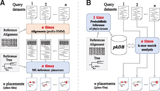
Comparison between existing PP software and RAPPAS. The pipelines from query sequence datasets to placement results (jplace files) are depicted. (A) Likelihood-based software requires, for each new query dataset, the step of aligning the query sequences to the reference alignment via an external tool (red box). The resulting extended alignment is the input for the PP itself (blue box). (B) RAPPAS builds a database of k-mers (the pkDB) once for a given reference tree and alignment. Many query datasets can then be placed without alignment, matching their k-mer content to this database. Each operation is run with a separate call to RAPPAS (blue boxes). (Color version of this figure is available at Bioinformatics online.)

To follow the standards defined by previous PP methods, the placements are reported in a JSON file following the ‘jplace’ specification (Matsen et al., 2012) (see Supplementary Material S1, Section S3, for more details). The results of RAPPAS can then be exploited in all jplace-compatible software, such as iTOL (visualization), Guppy (diversity analyses) or BoSSA (visualisation and diversity analysis) (Lefeuvre, 2018; Letunic and Bork, 2016; Matsen and Evans, 2013).

2.2 Construction of the pkDB

Before performing placements, a database of phylogenetically informative k-mers must be built; these ‘phylo-kmers’ are those that we would expect to see in a QS with non-negligible probability. The input for this phase is a reference alignment (denoted ‘refA’) and a reference tree (denoted ‘refT’) reconstructed from refA. The refT is interpreted as a rooted tree (as specified by the Newick file) and has lengths associated to its edges. This process is divided in three steps (see Fig. 2): (A) the injection of ‘ghost nodes’ on every edge of refT, (B) a process of ancestral state reconstruction based on this extended tree and (C) the generation of the phylo-kmers and their storage in a data structure.

Fig. 2.

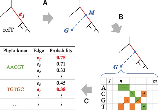
Construction of the pkDB. The construction of phylo-kmers for an edge is depicted (see the Section 2 for details.) (A) Each edge e₁ is bisected by a ghost node M, to which a terminal edge leading to another ghost node G is attached. (B) For each ghost node, a probability table for the sequence states expected at each site is generated using ancestral state reconstruction. (C) The most probable k-mers are computed from each table and then stored in the pkDB, together with the corresponding edge in the reference tree and the corresponding probability

The first step enables us to simulate evolution that has occurred and resulted in sequences not present in the reference alignment. For each edge of refT, a new edge branching off at its midpoint M is created (Fig. 2, Step A). The length of the new edge is set to the average length over all paths from M to its descendant leaves. The new leaves of these new edges (e.g. G in Fig. 2), and the midpoints M are referred to as ‘ghost nodes’. They represent unsampled sequences related to those in the reference alignment, whose most probable k-mers are the phylo-kmers. Note that the root of refT has an influence on computing the length of the newly added edges (e.g. from M to G in Fig. 2) as it determines the descendant leaves of each midpoint M. Although the position of the root is irrelevant to all other computations, it may have an effect on the quality of placements. If uncertain, we advise users to choose a root that has an ‘internal’ position within the reference tree (see Supplementary Material S1, Section S10).

The second step computes the probabilities necessary to the construction of the phylo-kmers. It is based on standard phylogenetic methods for ancestral sequence reconstruction (Fig. 2, Step B). Given refA, an alignment consisting of m sites over $S$ possible states (4 for DNA, 20 for amino acids), for each individual ghost node $G$ we compute an $S\times m$ table $(p_{\sigma ,j})$ of probabilities, where $p_{\sigma ,j}$ represents the marginal probability of state $\sigma$ at site $j$ (Yang et al., 1995). From this table, we compute the probabilities of any given k-mer at any ghost node $G$ (Fig. 2, Step C). Let $k$ be the chosen k-mer size (k = 8 by default) and let $n\in \{1,2,\dots ,m-(k-1)\}$be a particular site of refA. Assuming independence among sites (see, e.g. Felsenstein, 2004), the probability $P$ of k-mer ${\sigma }_1{\sigma }_2\dots {\sigma }_k$in $G$ at sites $\{n,n+1,\dots ,n+k-1\}$is given by:

$$P={\displaystyle \prod }_{i=1}^k{p}_{{\sigma }_i,n+i-1}$$

(1)

Each k-mer with a probability $P$ larger than a (parameterized) threshold (by default $1/S^k$⁠) is stored together with (i) the edge corresponding to the ghost node of origin, and (ii) the probability $P$ associated to this k-mer at the ghost node of origin (Fig. 2, Step C).

In the end, all the k-mers reconstructed above are stored in a data structure that allows fast retrieval of all relevant information associated to a k-mer, namely the list of edges for which it has high-enough probability, and the probabilities associated to each of these edges. This structure will be referred to as the phylo-kmers database (pkDB). We note that when the same k-mer is generated at different positions $n$ of refA, or at different ghost nodes for the same edge, only the highest probability is retained in the pkDB.

2.3 Placement algorithm

RAPPAS places each QS on the sole basis of the matches that can be found between the k-mers in the QS and the phylo-kmers stored in the pkDB. An algorithm akin to a weighted vote is employed: each k-mer in a QS casts multiple votes—one for each edge associated to that k-mer in the pkDB—and each vote is weighted proportionally to the logarithm of the k-mer probability at the voted edge (Supplementary Material S1, Section S1). The edge or edges receiving the largest total weighted vote are those considered as the best placements for a given QS.

A detailed description and complexity analysis for this algorithm can be found in Supplementary Material S1 Section S2. Unlike for alignment-dependent algorithms, the running time of RAPPAS does not depend on the length of the reference sequences, and rather than scaling linearly in the size of the reference tree, it only depends on the number of edges that are actually associated to some k-mer in the QS.

2.4 Accuracy experiments

The accuracy of the placements produced by RAPPAS and by competing likelihood-based PP software were evaluated following established simulation protocols (Berger et al., 2011; Matsen et al., 2010). Briefly, these protocols rely on independent pruning experiments, in which sequences are removed from refA and refT, and then used to generate QSs (we use the word read interchangeably, in these experiments), which are finally placed back to the pruned tree. The QSs are expected to be placed on the edge from which they were pruned. If the observed placement disagrees with the expected one, the distance between them is measured by counting the number of nodes separating the two edges. To make the placement procedure more challenging, we not only prune random reference taxa, but whole subtrees chosen at random. We consider this approach realistic in the light of current metagenomic challenges; because it is indeed common that large sections of the tree of life are absent from the reference phylogenies. The procedure was repeated for read lengths of 150, 300, 600 and 1200 bp. As in previous studies, the simulated reads are contiguous substrings of the pruned sequences obtained without introducing sequencing errors (Berger et al., 2011; Matsen et al., 2010). A detailed description of the procedure can be found in Supplementary Material S1, Section S4.

The impact of sequencing errors was evaluated independently. We repeated the procedure above on a single dataset (D652), and introduced errors in the simulated reads with the Mason read simulator (Holtgrewe, 2010) using the Illumina error model. Different rates (0.0, 0.1, 1 or 5%) were tested for two types of sequencing errors: substitutions and indels (detailed procedure and motivation found in Supplementary Material S1, Section S5).

2.5 Placement consistency on real-world data

As a complement to the experiments above, we also evaluated the placements of real-world reads on relatively large reference trees by reproducing the protocol described in Barbera et al. (2019). Because no proxy for the correct placement can be defined on these datasets, we evaluate the consistency between placements produced by RAPPAS and by the other methods. For each dataset (see Section 2.7 below) between 10 000 and 15 060 reads were placed on the reference tree using each method (EPA, EPA-ng, PPlacer and RAPPAS). For each pair of methods, the resulting placements were compared using the Phylogenetic Kantorovich–Rubinstein (PKR) metric (Evans and Matsen, 2012). Naturally, the lower the distance between two methods, the more similar the placements they produce are. We report median PKR-distances over all the placed reads, measured using the default behavior of each software (Supplementary Material S1, Section S6).

2.6 Runtime and memory experiments

CPU times were measured for each software with the Unix command time, using a single CPU core and on the same desktop PC (64GB of RAM, Intel i7 3.6 GHz, SSD storage). The fast aligner program hmmalign from HMMER (Eddy, 2011) was used to align the QSs to the refA, as in previous placement studies (Matsen et al., 2010). Placement runtimes were measured for two of the reference datasets that we describe in the next section, chosen so as to represent different combinations of the two parameters with the largest impact on runtimes (number of taxa and alignment length). Prior to starting the time measurement, for each dataset, GTR + Γ model parameters were estimated using RAxML. Then, dedicated options were used in EPA-ng and PPlacer to load these parameters and avoid optimization overheads (Supplementary Material S1, Section S9). Each software was launched independently three times and the median CPU time was retained. When available, masking options were kept as defaults. For EPA and EPA-ng, a single thread was explicitly assigned (option -T 1). PPlacer only uses a single thread and required no intervention. Default values were used for all other parameters. RAPPAS is based on Java 8+, which uses a minimum of 2 threads. We ensured fair comparison by using the Unix controller cpulimit, which aligns CPU consumption to the equivalent of a single thread (options –pid process_id –limit 100). For each RAPPAS process, memory was monitored by programmatically reading its usage at regular intervals.

2.7 Software and datasets used in experiments

The performance of RAPPAS (v1.00), both in terms of accuracy and computational efficiency, was compared against that of EPA (from RAxML v8.2.11) (Berger et al., 2011), PPlacer (v1.1alpha19) (Matsen et al., 2010) and EPA-ng (v0.3.4 for the experiments on real-world data and v0.2.0-beta for all other experiments) (Barbera et al., 2019).

Reference datasets (refA, refT) used for evaluating accuracy were taken from (Berger et al., 2011; Matsen et al., 2010) with the exception of D155, which was built for this study and corresponds to a whole genome alignment and tree for the hepatitis C virus. Each dataset is identified by the number of taxa present in the tree (e.g. D150 has 150 taxa). In total, 10 reference datasets were tested. Descriptive metadata reporting the nature of the locus, the length of the alignment and the gap content are displayed in Figure 3 (left headers) and Supplementary Material S2. One of the reference datasets (D140) is based on a reference alignment of protein sequences. Globally, the reference datasets represent a panel of loci commonly used in metabarcoding and metagenomic studies.

Fig. 3.

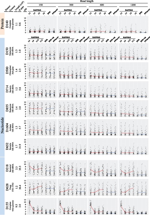
Accuracy comparison of RAPPAS and likelihood-based methods. Datasets corresponding to different marker genes or small genomes (left headers) were used to test placement accuracy for QSs of different lengths (top header). Lengths are measured in amino acids for D140 and in base pairs otherwise. Each gray box corresponds to a combination of dataset and QS length. In each box, the horizontal axis represents the tested software (RAPPAS was tested for several k-mer sizes), while the vertical axis corresponds to the measured node distance (ND) (the closer to 0, the more accurate the placement). For each software, each black dot represents the mean ND for one of the 100 independent pruning experiment (see Section 2) and white violins show the approximate distribution of the sample containing these 100 measures. The means of the four samples for RAPPAS are linked by a red line. The means of the three samples for the other methods are linked by a blue line. (Color version of this figure is available at Bioinformatics online.)

PKR distances between alternative placement methods were measured using five real world datasets: the three datasets available in Barbera et al. (2019) (named bv, neotrop, tara) and two large datasets of 5088 and 13 903 taxa (named green85 and LTP). The latter two datasets were retrieved from the Greengenes database (De Santis et al., 2006; release gg_13_8_otus, 85% OTUs tree) and the ‘All-Species Living Tree Project’ (Yilmaz et al., 2014; ssuRNA tree, release 132, June 2018), respectively. On the reference trees for green85 and LTP, we placed the QSs provided with the bv dataset, as they correspond to the same genetic region.

The runtime experiments are based on two of the above reference datasets, D652 (1.7 kbp) and D155 (9.5 kbp), and the QSs for placement were obtained in the following way. For D652, real-world 16S rRNA bacterial amplicons of about 150 bp were retrieved from the Earth Microbiome Project (Thompson et al., 2017) via the European Nucleotide Archive (Silvester et al., 2018) using custom scripts from github.com/biocore/emp/. Only sequences longer than 100 bp were retained. A collection of 3.1 × 10⁸ QSs were thus obtained. For D155, 10⁷ Illumina short reads of 150 bp were simulated from the 155 viral genomes in this reference dataset using the Mason read simulator (Holtgrewe, 2010). A substitution rate of 0.1% and very low indel rate of 0.0001% were chosen to avoid impacting negatively the runtime of the alignment phase for EPA, EPA-ng and PPlacer.

3 Results

3.1 Accuracy

The simulation procedure (see Section 2) was repeated for 10 different reference datasets representing genes commonly used for taxonomic identification. Accuracy is measured on the basis of the node distance between observed placement and expected placement (i.e. the number of nodes separating the two edges). The closer to zero the node distances are, the more accurate the method is. Figure 3 summarizes the results of the experiments for each choice of dataset, read length, and software. Each point in the plot shows the mean node distance for the reads generated by one pruned subtree of the reference tree. Each violin plot is based on as many points as there are pruned subtrees (i.e. 100). Horizontal lines link the per software node distance means, calculated as the mean of the 100 means above. Detailed mean values are reported in Supplementary Material S3.

As expected, given that they are based on the same general likelihood-based approach, EPA, EPA-ng, and PPlacer show very similar performance for all datasets and read lengths (Fig. 3, blue lines almost perfectly horizontal). As expected, the longer the reads are, the more accurate the placement is (Fig. 3, left to right boxes). The worst performances were observed for the D628 and D855 datasets, which agrees with previous studies (Berger et al., 2011; Matsen et al., 2010).

RAPPAS was subjected to the same tests using four k-mer sizes. The corresponding results can be classified into two groups. The first group contains the datasets for which using different values of k has a limited impact (Fig. 3, all except the last three). For these, RAPPAS shows globally an accuracy comparable to likelihood-based software. In simulations based on the shortest read lengths (Fig. 3, leftmost boxes) similar or even slightly better accuracies (leftmost boxes of D1604 and D652) are measured. On the other hand, the longest read lengths generally resulted in lower accuracy compared with other methods (rightmost boxes of D140, D150, D500, D855 and D1604).

The second group contains datasets where different values of k resulted in variable accuracy (Fig. 3, D218, D628 and D155). Two out of these three datasets are also characterized by a high proportion of gaps in their reference alignments (Fig. 3, left headers), which may be an adverse factor for the current version of RAPPAS (discussed below). Finally, D155, which corresponds to the longest reference alignment (9.5 kbp), is the only dataset where shorter k-mer sizes clearly lowered the accuracy of RAPPAS.

Figure 4 shows the accuracy loss measured on the D652 dataset after introducing different rates of sequencing errors in the simulation procedure (300 bp reads, k = 8 for RAPPAS). For all tested software, a very limited accuracy loss (≤0.2 node distance units) was measured for 0.1–1% substitutions/indel rates. Such error rates are typical for short read technologies (Glenn et al., 2011), suggesting that RAPPAS and all tested software are equally suitable for the placement of sequences produced by current technologies. When higher error rates are considered (5% substitutions/indels), RAPPAS appears to lose more accuracy than competing tools (Fig. 4, top rows and rightmost columns). Interestingly, indels appear to induce a higher accuracy loss than substitutions for every placement method tested. Different read lengths and different values of k for RAPPAS were also tested but showed similar trends (Supplementary Material S1, Section S5).

Fig. 4.

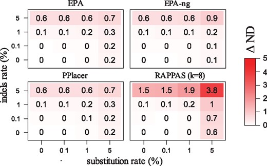
Accuracy loss in the presence of sequencing errors. Each square is a software tested under 16 conditions corresponding to varying rates of errors introduced into 300 bp reads (substitutions on the horizontal axis, indels on the vertical axis). Values represent the accuracy loss, calculated as the difference (Δ ND) between the mean node distance with indel/substitutions, and the mean node distance in the absence of sequencing errors (the bottom left condition with 0% indels, 0% substitutions)

3.2 Placement of real-world reads

The PKR distances measured for real-world reads placed on five medium-to-large reference trees are reported in Table 1. The question here is whether RAPPAS produces placements that can be viewed as strong outliers to those of the alignment-based methods. Note that some degree of difference is to be expected, given that RAPPAS has a radically different approach than the other methods. Another prediction is that PPlacer and EPA-ng should produce similar placements, as their default behavior includes similar heuristics aiming to reduce runtimes.

Table 1.

Median PKR distances over the placements of real-world reads on five different datasets

dataset	#taxa	pkDB		PKR distance
				PPlacer	EPA-ng	RAPPAS (k = 8)
neotrop	512	18 m 2.5GB	EPA	0.129	0.164	0.308
			PPlacer		0.048	0.247
			EPA-ng			0.310
bv	797	6 m 1.8GB	EPA	0.011	0.010	0.012
			PPlacer		0.002	0.005
			EPA-ng			0.004
tara	3748	30 m 9.7GB	EPA	0.076	0.073	0.175
			PPlacer		0.026	0.132
			EPA-ng			0.129
green85	5088	54 m 15.2GB	EPA	0.076	0.065	0.076
			PPlacer		0.006	0.045
			EPA-ng			0.030
LTP	13 903	5h18m 11.5GB	EPA	*	0.062	0.053
			PPlacer		*	*
			EPA-ng			0.086

Note: The lower the value, the closer the placements on the reference tree are between the two methods. The third column reports the time to build the pkDB (h, hours; m, minutes) and its size (GB, gigabytes) when using default parameters (k = 8). The distances for PPlacer on the LTP dataset are not reported (indicated by an asterisk) as this program reported numerical errors (see Supplementary Material S1, Section S6).

Consistent with the latter prediction, we observe that the PKR distances between PPlacer and EPA-ng are the smallest across all tested datasets. As for the former prediction (RAPPAS versus the other methods), for the tara and neotrop datasets, PKR distances between RAPPAS and the alignment-based methods are about two to three times higher than the average distance between the alignment-based methods. The difference, however, is much smaller for the other datasets. For the very large LTP dataset, we do not show the results of PPlacer, as it reported several warning messages and produced low-quality placements (see Supplementary Material S1, Section S6 for more detail).

3.3 Runtime

Figure 5 summarizes runtimes measured for the placement of 10³–10⁷ QSs on two reference datasets corresponding to short and long reference sequences (a marker gene for bacteria, and a complete virus genome, respectively). Figure 5A shows the times measured independently for each software. To consider the actual time needed in a scenario where a long-lifespan reference tree is used, in Figure 5B, the runtime reported for EPA, EPA-ng, and PPlacer includes both read alignment and placement, while the runtime of RAPPAS does not include pkDB construction (as the pkDB is already available).

Fig. 5.

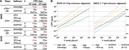
Placement runtime comparison. Runtimes were measured for a long (D155) and a short (D652) reference alignment, for a number of placement pipelines. (A) The execution time for each pipeline is decomposed into ‘preparation’ and “placement” steps. The preparation step for alignment-based methods is the alignment of each read to the reference (denoted ‘align’), while RAPPAS prepares a database once (noted ‘DB’). Runtimes for the analyses of 103 and 106 query reads are reported (h, hours; m, minutes), and for each read set the fastest combination of preparation plus placement is highlighted in red. (B) Boxes describe the placement runtime in a scenario where a long-lifespan pkDB is available (meaning that its construction needs not be repeated before the placement of a new query dataset). The horizontal axis reports the number of placed reads. The blue line shows the time used to align those reads to the reference dataset, the preliminary step required by alignment-based methods. For those methods, runtimes include the alignment phase (red and orange lines). (Color version of this figure is available at Bioinformatics online.)

As expected, EPA, PPlacer and EPA-ng show a runtime scaling linearly with the number of placed reads for both datasets (Fig. 5B). With the D155 dataset, EPA and PPlacer could not be run with a set of 10⁷ reads due to high memory requirements. Note that the runtime of EPA-ng for D155 is dominated by the time required to align the QSs (Fig. 5A).

The runtimes of RAPPAS appear to grow non-linearly when less than 10⁵ reads are placed due to the overhead imposed by loading the pkDB into memory. On the other hand, for larger read sets (≥10⁵) this overhead becomes negligible and the runtime of RAPPAS scales linearly with the number of reads. RAPPAS is much faster than the other methods. With D652, which is a short refA (Fig. 5B, right box), RAPPAS was up to 5 × faster than EPA-ng (5.0 × for k = 12 and 2.4 × for k = 8) and up to 53 × faster than PPlacer (52.7x for k = 12 and 26.3 × for k = 8). With D155, which is a longer refA (Fig. 5B, left box), greater speed increases are observed: RAPPAS was about 40 × faster than EPA-ng (36.9 × for k = 8 and 38.9 × for k = 12) and about 130x times faster than PPlacer. Concretely, using a single CPU and a common desktop computer, RAPPAS is capable to place one million 100–150 bp DNA reads in 30 min on D652 and in 11 min on D155.

3.4 Implementation

RAPPAS is distributed as a standalone command-line application. It is compatible with any system supporting Java 1.8+. Ancestral sequence reconstruction is performed via an external program. Currently PhyML 3.3+ (Guindon et al., 2010) and PAML 4.9 (Yang, 2007) binaries are supported by RAPPAS. The main limiting factor for RAPPAS is the amount of memory required to build the pkDB (and subsequently, to load the pkDB for the placement phase). Figure 6 reports the memory and drive storage requirements related to building and storing the pkDB for three representative datasets and different values of k. D150 (few taxa, short alignment), D155 (few taxa, long alignment) and D1604 (many taxa, short alignment) show memory usage below 4GB for k = 10, and 12GB for k = 12, which indicates that RAPPAS can be launched on most standard laptop computers, if k is set to a low value. A Git repository, instructions to compile RAPPAS and tutorials are available at https://gite.lirmm.fr/linard/RAPPAS.

Fig. 6.

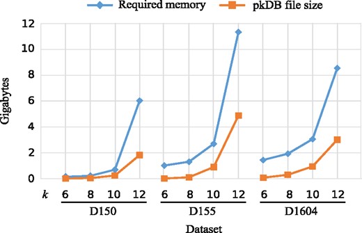
Memory and storage requirements related to the pkDB. Memory and storage requirements of RAPPAS are reported for three datasets, representative of different combinations of number of taxa and alignment length (D150, 1.3 kbp; D155, 9.5 kbp; D1604, 1.3 kbp). The blue line reports the memory peaks experienced during pkDB construction. The orange line displays the size of the pkDB when saved as a compressed binary file. (Color version of this figure is available at Bioinformatics online.)

4 Discussion

4.1 Advantages of alignment-free placements

The novel algorithm introduced in RAPPAS removes a major limitation imposed by previous PP software: these methods rely on the computation of a multiple alignment merging the reference alignment and query sequences, a step which must be repeated for each new set of query sequences (Fig. 2A). The idea of attaching k-mers to pre-computed metadata to accelerate sequence classification has been explored by algorithms combining taxonomically informed k-mers and LCA-based classification (Liu et al., 2018; Müller et al., 2017; Ounit et al., 2015; Wood and Salzberg, 2014). However, none of these methods have the goal of producing evolutionarily precise classifications based on probabilistic models of sequence evolution. RAPPAS adapts this idea to PP by reconstructing sets of probable, phylogenetically informed k-mers, called phylo-kmers.

When compared with previous PP methods, RAPPAS has two critical algorithmic advantages (see Supplementary Material S1, Section S2 for details). First, its runtime does not depend on the length of the reference alignment, since the sequences in the reference tree, and those that are related to them, are summarized by their phylo-kmers. Note that the alignment phase required by the other PP methods has a runtime that scales linearly with the length of refA (if profile alignment is used; Eddy, 1998). Second, while the placement runtime of other PP methods is linear in the number of reference taxa (i.e. the size of refT) (Matsen et al., 2010), for RAPPAS it depends only on the number of edges associated to the queried phylo-kmers, which may be significantly smaller than the number of taxa. This second property has limited impact for a small refT with very similar reference sequences, or for small values of k (as k-mers will be assigned to many tree edges), but is favorable for a large refT, spanning a wide taxonomic range, and large values of k (as k-mers will be assigned to a low proportion of the edges).

Our experiments on two reference datasets with very different combinations of the parameters governing runtimes (number of taxa and alignment length) show that, on real data, the initial implementation of RAPPAS is already faster than alternative PP pipelines (Fig. 5). This includes EPA-ng that, despite being based on low level optimizations (e.g. CPU instructions, optimized libraries etc.) (Barbera et al., 2019), is only faster than RAPPAS when few query sequences are analysed. As expected, the speed gain provided by the alignment-free approach appears to be more pronounced for long reference alignments (Fig. 5B, left box). Finally, while the present implementation is based on a single thread, most steps of RAPPAS should be fully parallelizable, offering even faster placements in the future.

4.2 Accuracy limitations and future work

The presence of dense gappy regions in refA appears to have a negative impact on the accuracy of RAPPAS, especially in combination with larger k-mer sizes: D218 and D628 are the most gappy of the tested datasets and cause increasingly worse accuracy (compared with EPA/PPlacer) when k increases from 8 to 12 (Fig. 3). The likely reason behind this limitation is the following. As is standard practice in phylogenetics, substitution models used for ancestral state reconstruction do not treat gaps in refA as sequence states. As a result, our phylo-kmers are sequences composed of nucleotides (or amino acids) only and cannot be used to model the presence of indels in the query sequences. The by-default construction of phylo-kmers described in the Methods produces phylo-kmers that will not match the query sequences having indels among the corresponding positions. Clearly, the longer the k-mers are, the more likely these failed matches are to occur. A possible solution to this issue consists of recording the coordinates of the indels present in refA, and generate phylo-kmers that skip the refA intervals defined by those coordinates. This solution is implemented in RAPPAS, and we describe it in more detail in Supplementary Material S1, Section S8. Other improvements may be possible, e.g. allowing inexact (approximate) matching between the query and the stored k-mers, as explored in several k-mer based sequence classification tools (Břinda et al., 2015; Müller et al., 2017) or in tools for sequence comparison (Horwege et al., 2014). These or other solutions, adapted to a probabilistic setting, will be examined in the future to reduce the sensitivity of RAPPAS to gaps.

Another limitation of RAPPAS is that although it is practically as accurate as likelihood-based methods for read lengths that are commonly produced by Illumina sequencing (e.g. 150–300 bp), it tends to become less accurate on longer reads (Fig. 3). This is not surprising: query sequences are treated by RAPPAS as unordered collections of k-mers, meaning that RAPPAS does not evaluate whether the matches between the phylo-kmers and the query k-mers respect some form of positional consistency or collinearity. It is intuitive that this problem is potentially more harmful to accuracy for longer query sequences. Since long read sequencing is developing rapidly, future versions of the algorithm will deal with this issue by taking into account the positions within refA from which the phylo-kmers originated.

We note that low values of k and long reference alignments make it possible for the same phylo-kmer to be generated at more than one position in refA. Frequent occurrence of this event may have an undesired impact on the placement score of reads, and ultimately affect placement accuracy. This is the likely reason for the lower accuracy observed in the D155 dataset (especially for k = 6), which corresponds to a complete viral genome rather than a single short genetic marker (Fig. 3, lowest row).

The choice of the value of k should be made on the basis of the available computational resources, in particular memory. Larger values of k lead to larger pkDBs that require more memory. Currently, the default value for k is set to 8, as this appears to ensure a good combination of placement accuracy (Fig. 3), and memory requirements (Fig. 6 and Table 1). The choice of k is an issue that applies to all k-mer based methods, and very few approaches to automatically adapt k to the data at hand have been proposed, for example for genome assembly (Shariat et al., 2014). In the case of PP, this may entail runtime-expensive analyses such as pruning experiments based on the reference dataset at hand (producing accuracy estimates for several values of k, as in Fig. 3). Future releases of RAPPAS may include a module allowing advanced users to test different values of k prior to pkDB construction.

When placing real-world reads, for most of the tested datasets, RAPPAS produced placements relatively similar to the other methods (Table 1). The differences observed in the tara and the neotrop dataset are probably due to the radically different approaches of RAPPAS and alignment-based methods. We observed that the tara dataset is characterized by a gappy reference alignment, which may impact RAPPAS placements, as described above. The neotrop refA is not only gappy, but also gives a reference tree that is very non-clocklike (the leaves are at very different distances from the root), which may also impact RAPPAS, as the branch lengths set at ghost node construction are conceived for data consistent with a molecular clock.

4.3 Conclusion

The design principle behind RAPPAS (Fig. 1) is particularly adapted to metagenomic analyses based on standardized references (trees and alignments) with a long lifespan. This applies to the context of medical diagnostics where, for instance, virus ‘typing’ aims to classify viral reads within group-specific standardized references (Sharma et al., 2015). The references are built and manually curated by specialized teams, and may become standard for months to years in these medical communities (Kroneman et al., 2011). Similarly, databases of standard prokaryotic and eukaryotic markers, such as EukRef (Del Campo et al., 2018), SILVA (Quast et al., 2012), RDP (Cole et al., 2014), PhytoRef (Decelle et al., 2015) and Greengenes (De Santis et al., 2006), are widely used for taxonomic classification. pkDBs for such references can be built once and shared broadly, allowing many users to efficiently identify a sample’s composition with RAPPAS, without the need for rebuilding the database or aligning the sampled reads.

Although Section 4.2 discusses potential improvements to placement accuracy, the computational efficiency of RAPPAS will also be a central focus of our future work. For example, tailored k-mer indexing techniques can be developed similarly to other recent work (Liu et al., 2018; Müller et al., 2017), and the memory footprint of the pkDB can be reduced by limiting storage to the most discriminant phylo-kmers (Ounit et al., 2015). Despite the potential improvements to RAPPAS, it is already faster than other PP implementations on real datasets (Fig. 5). As the RAPPAS algorithm evolves to place query sequences with increased efficiency and accuracy (especially for longer queries), it will open the door to PP as a means to standardized diagnostic species identification.

Acknowledgements

We would like to thank Olivier Gascuel for helpful advice, as well as Anne-Mieke Vandamme, Krystof Theys, Pieter Libin, Frédéric Mahé and Jakub Truszkowski for sharing data and fruitful discussions. BL is also grateful to Vincent Lefort for his everyday advice. Finally, we thank A. Stamatakis, P. Barbera and an anonymous reviewer for their constructive comments which helped improve the article. B.L., K.S. and F.P. conceived of the study; B.L., K.S. and F.P. designed the algorithm; B.L. coded the software; B.L., K.S. and F.P. wrote the article.

Funding

This work has been supported by the European Union’s Horizon 2020 research and innovation program under grant agreement [No 634650] (Virogenesis.eu). BL was also supported by three Labex: Labex Agro [ANR-10-LABX-0001–01], Labex CeMEB [ANR-10-LABX-0004] and Labex NUMEV [ANR-10-LABX-20].

Conflict of Interest: none declared.