Compositional data network analysis via lasso penalized D-trace loss

Abstract

Motivation

With the development of high-throughput sequencing techniques for 16S-rRNA gene profiling, the analysis of microbial communities is becoming more and more attractive and reliable. Inferring the direct interaction network among microbial communities helps in the identification of mechanisms underlying community structure. However, the analysis of compositional data remains challenging by the relative information conveyed by such data, as well as its high dimensionality.

Results

In this article, we first propose a novel loss function for compositional data called CD-trace based on D-trace loss. A sparse matrix estimator for the direct interaction network is defined as the minimizer of lasso penalized CD-trace loss under positive-definite constraint. An efficient alternating direction algorithm is developed for numerical computation. Simulation results show that CD-trace compares favorably to gCoda and that it is better than sparse inverse covariance estimation for ecological association inference (SPIEC-EASI) (hereinafter S-E) in network recovery with compositional data. Finally, we test CD-trace and compare it to the other methods noted above using mouse skin microbiome data.

Availability and implementation

The CD-trace is open source and freely available from https://github.com/coamo2/CD-trace under GNU LGPL v3.

Supplementary information

Supplementary data are available at Bioinformatics online.

1 Introduction

Microbes play an important role in the environment and human life. Bacteria have been found in many parts of the biosphere, including some extreme conditions such as deep sea vents with high temperatures and rocks of boreholes beneath the Earth’s surface (Pikuta et al., 2007). Micro-organisms are also significant for Earth’s biogeochemical cycles by participating in decomposition, carbon and nitrogen fixation and oxygen production. In the human body, it is estimated that the number of microbe cells is about 10 times that of the human cells (Zoetendal et al., 2004). These microbes affect human health and well-being (Gill et al., 2006). However, microbes affect human health in ways we have only begun to explore. Analysis of the human microbiome may help us to better understand our own genome.

Sequencing technologies have increased in quality, while cost has decreased, providing an opportunity to analyze microbial communities through sequencing data. This represents a substantial improvement over traditional microbial studies, which are hindered by several limiting factors. First, only a small proportion of microbes can be cultured under laboratory conditions. Second, while only single microbes can be studied in laboratories, it is well known that most microbes survive and interact with other microbes, making it correspondingly difficult to draw firm conclusions from lab studies. In contrast, sequencing technologies allow researchers to collect information from the whole genomes of all microbes in a community directly from their natural environment, facilitating mixed genomic surveys (Handelsman et al., 1998).

Microbes are often represented by common operational taxonomic units (OTUs) after grouping sequencing reads of variable regions of 16S-rRNA genes (Wooley et al., 2010). The abundances of the underlying microbial species are quantified by counting OTUs. However, these counts are usually converted into compositional data such as proportions based on total counts in one sample, which only represent the relative abundances of microbial species, to limit the biases resulting from different collection scales and various sequencing depths. This feature of microbiome data is called compositionality. Compositional data present unique challenges for statistical analysis, since restriction of the constant sum can bring spurious results if it is ignored [e.g. correlation analysis (Pearson, 1896)]. In addition, microbiome data are considered high-dimensional, where the number of measured OTUs is often greater than the sample size. Such high dimensionality also presents statistical challenges for statistical inference, such as the inference of inverse covariance (Friedman, 2008; Meinshausen and Bühlmann, 2006; Yuan and Lin, 2006).

In ecological studies, we should be able to infer microbial interaction networks in specific environments based on high-dimensional and compositional microbiome data (Faust et al., 2012; Weiss et al., 2016). Indeed, several methods have been proposed to infer the correlation network for microbiome studies (Fang et al., 2015; Faust et al., 2012; Friedman and Alm, 2012). However, compared with pair-wise correlation dependencies that include both direct and indirect interactions, researchers are often more concerned with conditional dependencies which only describe direct interactions (Friedman, 2004). Biswas et al. (2016) proposed an algorithm called MInt to learn direct interactions based on a Poisson-multivariate normal hierarchical model from microbiome sequencing experiments. However, MInt does not explicitly account for the compositional nature of microbiome data. Kurtz et al. (2015) proposed an approximate method called SPIEC-EASI (S-E) to infer direct interactions in microbiome studies. The key assumption of S-E is that the covariance matrix of the absolute abundances can be approximated by the covariance matrix of the compositions after the centered log-ratio (clr) transformation, when the number of microbes is large enough. Yang et al. (2016) used a hierarchical Bayesian statistical model called mLDM to infer sparse microbial interactions. However, mLDM introduces too many parameters, limiting its scalability and efficiency to dimensionality cases. Fang et al. (2017) proposed a method called gCoda to estimate sparse direct interactions by penalizing the likelihood function of compositional data. The main difficulty for gCoda is the non-convexity of the likelihood function.

Therefore, in this paper, we introduce a novel empirical loss function for compositional data called compositional D-trace(CD-trace) loss, based on D-trace (Zhang and Zou, 2014) which estimates high-dimensional sparse precision matrices and proposes a new loss function, termed D-trace loss. According to the authors, a novel sparse precision matrix estimator, or inverse covariance matrix with absolute abundance data, is obtained by minimizing lasso penalized D-trace loss under a positive-definiteness constraint. The rest of the paper is organized as follows. In Section 2, we introduce the proposed compositional D-trace(CD-trace) loss function and the constrained penalized loss minimization framework for direct interaction network estimation. We also develop an efficient algorithm for numerical computation based on the alternating direction algorithm. In Section 3, we evaluate the performance of our method by comparing CD-trace with other state-of-the-art methods under different simulation settings. The proposed method is further used to conduct network recovery with mouse skin microbiome data.

2 Materials and methods

2.1 Notations about composition data

Assume D microbe species with absolute abundances $\mathit{z}=\text{exp}(\mathit{w})=(\text{exp}(w_1),\hspace{0.17em}\hspace{0.17em}\text{exp}(w_2),\hspace{0.17em}\dots ,\hspace{0.17em}\hspace{0.17em}\text{exp}(w_D))$ respectively, where $\mathit{w}=\text{log}(\mathit{z})=(w_1,w_2,\dots ,w_D)$ is the log-transformed absolute abundance. Further assume that absolute abundances w follow a multivariate normal distribution with mean $\mathit{\mu }$ and non-singular covariance matrix Σ. Then the precision matrix $\Theta ={\Sigma }^{-1}$ fully characterizes the direct interactions among microbial species (Whittaker, 1990). More specifically, the i-th species and j-th species are independent given other species if and only if the (i, j) element of the precision matrix is 0 (Friedman, 2004). Thus, an important goal of microbial ecology study is to infer the precision matrix Θ or the microbial interaction network. If the absolute abundances $\mathit{z}=\text{exp}(\mathit{w})$ are known, then the precision matrix Θ can be estimated with methods such as graphical lasso or D-trace directly. However, in real biological experiments, it is often the case that only relative abundances or compositions

$$x_i=\frac{z_i}{{\sum }_{k=1}^D{z}_k}=\frac{\hspace{0.17em}\text{exp}(w_i)}{{\sum }_{k=1}^D\hspace{0.17em}\text{exp}\hspace{0.17em}(w_k)},i=1,2,\dots ,D$$

(1)

can be observed, not the absolute abundances $\text{exp}(\mathit{w})$⁠, making absolute abundances w become latent variables. Here, we aimed to estimate the precision matrix Θ among latent variable w from the observed relative abundances x instead of the unobserved absolute abundances.

A naive method of inferring the precision matrix with compositional data involves ignoring the compositionality and simply applying graphical lasso to the log-transformed compositions $\ln \mathbf{x}$⁠. We can illustrate the poor performance of this naive method with a simple example. We partition 51 species into 3 disjoint groups evenly and select a hub for each group. Each hub is connected to other nodes in the same group with strengths distributed in [−0.2, 0.2] uniformly. Thus we get a 3-hub graph Θ. Absolute abundances w are generated having the normal distribution with mean $0_{51}$ and covariance ${\Theta }^{-1}$⁠, and then x is computed according to (1). We consider four sample sizes $n=100,200,500,1000$⁠, and use graphical lasso to $\ln \mathrm{x}$ in order to recover the precision matrix. The corresponding receiver operating characteristic (ROC) curves are shown in Figure 1 for each sample size. Poor performance is revealed when the method fails to recover the network, even when the sample size is very large. This example demonstrates the risk of ignoring compositionality in network inference.

Fig. 1.

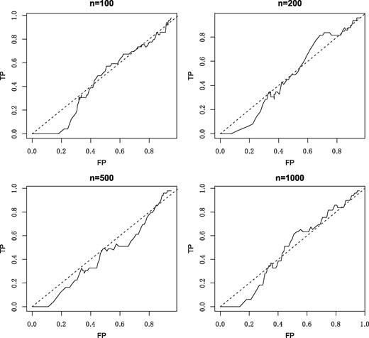
ROC curve for different sample sizes with the naive method

The clr transformation (Aitchison, 1981) is often used in the analysis of compositional data. The clr transformation matrix $F=I-\frac{1}{D}{\mathbf{1}}_{\mathit{D}}{1}_{\mathit{D}}^T$ satisfies $\text{Rank}(F)=D-1,F{\mathbf{1}}_{\mathit{D}}=0$ and $F^2=F$⁠, where I is the identity matrix and ${\mathbf{1}}_{\mathit{D}}$ is a D-dimensional all-ones vector. The data with clr transformation are $F \ln \mathit{x}=F\mathit{w}-\ln ({\sum }_{k=1}^D\hspace{0.17em}\text{exp}\hspace{0.17em}(w_k))F{\mathbf{1}}_{\mathit{D}}=F\mathit{w}$⁠. The corresponding covariance matrix is

$$F\hspace{0.17em}\text{Var}(\ln \mathit{x})F=F\hspace{0.17em}\text{Var}(\mathit{w})F$$

(2)

where $\text{Var}(\ln \mathit{x})$ and $\text{Var}(\mathit{w})$ are the covariance matrix of $\ln \mathit{x}$ and w, respectively. Equation (2) is an important bridge between the covariance matrix of log-transformed relative abundances (or compositions) and absolute abundances. In the following section, we introduce a loss function to estimate the precision matrix Θ among the latent variable w from the compositional data by utilizing this bridge.

2.2 The D-trace loss function

We start with some notations and definitions for convenience. Suppose that $A=(A_{i,j})\in {\mathcal{R}}^{D\times D}$ is a D × D matrix. Then, we denote $\left|\right|A|{|}_{\mathrm{F}}={(\sum _{i,j}{A}_{i,j}^2)}^{1/2}$ as its Frobenius norm and $\left|\right|A|{|}_{1,\text{off}}=\sum _{i\cancel{=}j}|A_{\mathit{ij}}|$ as the off-diagonal ${\ell }_1$ norm. The transposition and trace of A is denoted as $A^{\mathrm{T}}$ and tr(A), respectively. Let vec(A) be the D²-vector by stacking the columns of A. For two symmetric matrices $X,Y\in {\mathcal{R}}^{D\times D},\hspace{0.17em}X\succcurlyeq Y$ means that X – Y is positive semi-definite, and $X\succ 0$ means that X is positive definite. We use $\langle X,Y\rangle$ to denote $\mathit{tr}(X{Y}^{\mathrm{T}})$ in this paper and we have $\langle A,A\rangle =\left|\right|A|{|}_{\mathrm{F}}^2$⁠.

Importantly, our goal is to estimate the precision matrix Θ with the observed compositional data instead of the otherwise unattainable absolute abundances. Similar to Zhang and Zou (2014), we want to construct a new convex loss function $L(\Theta ,\Sigma )$ such that its unique minimizer for the given Σ is achieved at $\Theta ={\Sigma }^{-1}$⁠. In other words, the minimizer of the loss function $L(\Theta ,\Sigma )$ should satisfy $\Theta \Sigma =I$⁠. Consider the following loss function

$$L_D(\Theta ,\Sigma )=\frac{1}{4}(\langle F\Theta ,\Theta F\Sigma F\rangle +\langle F\Sigma F\Theta ,\Theta F\rangle )-\langle \Theta ,F\rangle$$

(3)

as the D-trace loss function for compositional data. It is easy to check that

$$\begin{array}{c}L({\Theta }_1,\Sigma )+L({\Theta }_2,\Sigma )-2L(\frac{{\Theta }_1+{\Theta }_2}{2},\Sigma )\\ =\frac{1}{8}\langle F({\Theta }_1-{\Theta }_2),({\Theta }_1-{\Theta }_2)F\Sigma F\rangle \\ +\frac{1}{8}\langle F\Sigma F({\Theta }_1-{\Theta }_2),({\Theta }_1-{\Theta }_2)F\rangle \ge 0\end{array}$$

holds for D × D symmetric matrices ${\Theta }_1,\hspace{0.17em}{\Theta }_2$⁠, which implies that $L_D(\Theta ,\Sigma )$ is convex as a function of Θ for a given Σ. To find the minimizer of (3) for a given Σ, we show that the derivation of $L_D(\Theta ,\Sigma )$ with respect to Θ is

$$\frac{\partial L_D}{\partial \Theta }=(F\Theta F\Sigma F+F\Sigma F\Theta F)/2-F.$$

(4)

If the covariance matrix Σ and the clr transformation matrix is exchangeable, namely

$$F\Sigma =\Sigma F,$$

(5)

then the derivation in Equation (4) can be written as

$$\frac{\partial L_D}{\partial \Theta }=\frac{1}{2}F(\Theta \Sigma +\Sigma \Theta -2I)F.$$

(6)

It is easy to see that $\Theta ={\Sigma }^{-1}$ solves Equation (6). Therefore, it is also a minimizer of $L_D(\Theta ,\Sigma )$ since $L_D(\Theta ,\Sigma )$ is convex.

The exchangeable condition in Equation (5) is equivalent to ${\mathbf{1}}_{\mathit{D}}{1}_D^T\Sigma =\Sigma {\mathbf{1}}_{\mathit{D}}{1}_{\mathit{D}}^T$ or $\sum _l\text{Cov}(w_i,w_l)$ = $\sum _l\text{Cov}(w_j,w_l)$ for all $i,j=1,2,\dots ,D$⁠, which is similar to the condition in Sparse Correlations for Compositional data (SparCC), as Friedman and Alm (2012) proposed to infer the pair-wise correlations of basis abundance rather than their proportions. They assume that $\sum _{l\cancel{=}i}\text{Cov}(w_i,w_l)=0,i=1,2,\dots ,D$⁠. To elucidate the nature of the two assumptions, consider the special case where $\text{Var}(w_i),i=1,2,\dots ,D$ are the same. Then our exchangeable condition simplifies to $\sum _{l\cancel{=}i}\text{Cor}(w_i,w_l),i=1,2,\dots ,D$ is the same, in other words, the average correlation with other species is nearly the same for each species. Similarly, the assumption in SparCC simplifies to $\sum _{l\cancel{=}i}\text{Cor}(w_i,w_l)=0,i=1,2,\dots ,D$⁠, namely, the average correlation is very small. We see that our condition is weaker than the assumption in SparCC in this special case.

At the end of this section, we point out another advantage of the proposed loss function. Although we cannot estimate the covariance matrix $\Sigma =\text{Var}(\mathit{w})$ in loss function (3) from the observed relative abundances x directly, we can estimate $F\Sigma F=F\text{Var}(\ln \mathit{x})F$ [Equation (2)] since $\text{Var}(\ln \mathit{x})$ can be easily estimated with the finite sample covariance matrix.

2.3 Lasso penalized estimator

In real applications, by plugging in the finite sample covariance matrix of $\text{Var}(\ln \mathit{x})$ and using the bridge described in the last section, we get the empirical version of CD-trace loss

$$L_D(\Theta )=\frac{1}{4}(\langle F\Theta ,\Theta F{\widehat{\Sigma }}_{\ln x}F\rangle +\langle F{\widehat{\Sigma }}_{\ln x}F\Theta ,\Theta F\rangle )-\langle \Theta ,F\rangle .$$

(7)

The sparse assumption holds that the direct interaction network is sparse when D is large; in this case, we incorporate the ${\ell }_1$ penalty (Tibshirani, 1996) on the off-diagonal elements of Θ into CD-trace loss. Hence, our estimator for the precision matrix is proposed as

$$\widehat{\Theta }=\underset{\Theta \succ 0}{\text{argmin}}{L}_D(\Theta )+\lambda \left|\right|\Theta |{|}_1,$$

(8)

where $\lambda >0$ is a tuning parameter. We develop an efficient alternating direction method of multipliers (ADMM) (Boyd et al., 2011) to solve the objective function (8) in Section 2.4. Following the idea of Zhao et al. (2014), we select the tuning parameter by minimizing the Bayesian Information Criterion (BIC) (Schwarz et al., 1978), as

$$\text{BIC}=n\left|\right|F\Theta F{\widehat{\Sigma }}_{\ln x}F+F{\widehat{\Sigma }}_{\ln x}F\Theta F)/2-F|{|}_1+\text{log}(n)|\Theta {|}_0,$$

where $|\Theta {|}_0$ is the number of non-zero elements in the upper-triangle of Θ and n is the sample size.

2.4 Algorithm

Directly minimizing the objective function (3) is difficult; therefore, we first introduce four auxiliary matrices Θ_i,$i=1,2,3,4$⁠, and rewrite (8) as

$$\underset{{\Theta }_1={\Theta }_2={\Theta }_3={\Theta }_4}{\text{argmin}}{L}_1({\Theta }_1)+L_2({\Theta }_2)+\lambda \left|\right|{\Theta }_3|{|}_{1,\text{off}}+h({\Theta }_4\succcurlyeq ϵI)$$

(9)

where $L_1({\Theta }_1)=\frac{1}{4}\langle F{\Theta }_1,{\Theta }_{1}F{\widehat{\Sigma }}_{\ln x}F\rangle -\frac{1}{2}\langle {\Theta }_1,F\rangle ,\hspace{0.17em}{L}_2({\Theta }_2)=\frac{1}{4}\langle F{\widehat{\Sigma }}_{\ln x}F{\Theta }_2,{\Theta }_{2}F\rangle -\frac{1}{2}\langle {\Theta }_2,F\rangle$ and $h({\Theta }_4\succcurlyeq ϵI)$ is an indicator function defined by

$$h({\Theta }_4\succcurlyeq ϵI)=\{\begin{array}{cc}0\hfill & {\Theta }_4\succcurlyeq ϵI,\hfill \\ \infty \hfill & \text{otherwise}.\hfill \end{array}$$

(10)

Note that solving (9) is equivalent to minimizing (8) since $L_D(\Theta )=L_1(\Theta )+L_2(\Theta )$⁠. The auxiliary matrices ${\Theta }_3$ and ${\Theta }_4$ are introduced to handle the ${\ell }_1$ penalty and positive-definite constraint in (8). Consider the following augmented Lagrangian function

$$\begin{array}{c}L({\Theta }_1,{\Theta }_2,{\Theta }_3,{\Theta }_4,{\Lambda }_1,{\Lambda }_2,{\Lambda }_3,{\Lambda }_4,{\Lambda }_5)\\ =L_1({\Theta }_1)+L_2({\Theta }_2)+\lambda \left|\right|{\Theta }_3|{|}_{1,\text{off}}+h({\Theta }_4\succcurlyeq ϵI)\\ +<{\Lambda }_1,{\Theta }_3-{\Theta }_1>+<{\Lambda }_2,{\Theta }_2-{\Theta }_3>\\ +<{\Lambda }_3,{\Theta }_1-{\Theta }_2>+<{\Lambda }_4,{\Theta }_4-{\Theta }_1>\\ +<{\Lambda }_5,{\Theta }_2-{\Theta }_4>+(\rho /2)\left|\right|{\Theta }_3-{\Theta }_1|{|}_{\mathrm{F}}^2\\ +\hspace{0.17em}(\rho /2)\left|\right|{\Theta }_2-{\Theta }_3|{|}_{\mathrm{F}}^2+(\rho /2)||{\Theta }_1-{\Theta }_2|{|}_{\mathrm{F}}^2\\ +\hspace{0.17em}(\rho /2)\left|\right|{\Theta }_1-{\Theta }_4|{|}_{\mathrm{F}}^2+(\rho /2)||{\Theta }_2-{\Theta }_4|{|}_{\mathrm{F}}^2,\end{array}$$

(11)

where ρ is a given positive real number and ${\Lambda }_1,{\Lambda }_2,{\Lambda }_3$ are Lagrangian multipliers. Following the idea of ADMM algorithm, we can solve (11) by updating ${\Theta }_1,{\Theta }_2,{\Theta }_3,{\Theta }_4,{\Lambda }_1,{\Lambda }_2,{\Lambda }_3,{\Lambda }_4,{\Lambda }_5$ iteratively. Specifically, given ${\Theta }_1^k,\hspace{0.17em}{\Theta }_2^k,\hspace{0.17em}{\Theta }_3^k,\hspace{0.17em}{\Theta }_4^k$ and ${\Lambda }_1^k,\hspace{0.17em}{\Lambda }_2^k,\hspace{0.17em}{\Lambda }_3^k,\hspace{0.17em}{\Lambda }_4^k,\hspace{0.17em}{\Lambda }_5^k$ at the k-th step, the estimators are updated alternately according to

$${\Theta }_1^{k+1}=\underset{{\Theta }_1}{\text{argmin}}L({\Theta }_1,{\Theta }_2^k,{\Theta }_3^k,{\Theta }_4^k,{\Lambda }_1^k,{\Lambda }_3^k,{\Lambda }_4^k)$$

(12)

$${\Theta }_2^{k+1}=\underset{{\Theta }_2}{\text{argmin}}L({\Theta }_1^{k+1},{\Theta }_2,{\Theta }_3^k,{\Theta }_4^k,{\Lambda }_2^k,{\Lambda }_3^k,{\Lambda }_5^k)$$

(13)

$${\Theta }_3^{k+1}=\underset{{\Theta }_3}{\text{argmin}}L({\Theta }_1^{k+1},{\Theta }_2^{k+1},{\Theta }_3,{\Lambda }_1^k,{\Lambda }_2^k)$$

(14)

$${\Theta }_4^{k+1}=\underset{{\Theta }_4}{\text{argmin}}L({\Theta }_1^{k+1},{\Theta }_2^{k+1},{\Theta }_4,{\Lambda }_4^k,{\Lambda }_5^k)$$

(15)

$$\begin{array}{c}{\Lambda }_1^{k+1}={\Lambda }_1^k+\rho ({\Theta }_3^{k+1}-{\Theta }_1^{k+1})\\ {\Lambda }_2^{k+1}={\Lambda }_2^k+\rho ({\Theta }_2^{k+1}-{\Theta }_3^{k+1})\\ {\Lambda }_3^{k+1}={\Lambda }_2^k+\rho ({\Theta }_1^{k+1}-{\Theta }_2^{k+1})\\ {\Lambda }_4^{k+1}={\Lambda }_4^k+\rho ({\Theta }_4^{k+1}-{\Theta }_1^{k+1})\\ {\Lambda }_5^{k+1}={\Lambda }_5^k+\rho ({\Theta }_2^{k+1}-{\Theta }_4^{k+1}).\end{array}$$

(16)

The explicit solutions to the above optimization problems and the detailed proofs are found in the Supplementary Material. We summarize this ADMM algorithm in the following Algorithm 1. The convergence of Algorithm 1 is guaranteed by the convergence theory for alternating direction method provided by Boyd et al. (2011). In our simulations and real data analysis, we take ρ = 50 and terminate the algorithm if $\left|\right|{\Theta }_j^{k+1}-{\Theta }_j^k|{|}_{\mathrm{F}}<{10}^{-3}\max (1,\left|\right|{\Theta }_j^k|{|}_{\mathrm{F}},|\left|{\Theta }_j^{k+1}\right|{|}_{\mathrm{F}}),j=1,2,3,4$⁠.

Algorithm 1. The ADMM algorithm for the lasso penalized D-trace loss estimator.

Initialization: k=0, let ${\Theta }_1^{\mathrm{0}},{\Theta }_2^{\mathrm{0}},{\Theta }_3^{\mathrm{0}},{\Theta }_4^{\mathrm{0}}={(F\widehat{\Sigma }F+5I)}^{-1}$⁠, and $\Lambda 1^0,{\Lambda }_2^{\mathrm{0}},{\Lambda }_3^{\mathrm{0}},{\Lambda }_4^{\mathrm{0}},{\Lambda }_5^{\mathrm{0}}$ to be zero matrix.

Given ${\Theta }_i^k,\hspace{0.17em}i=1,2,3,4$ and ${\Lambda }_i^k,\hspace{0.17em}i=1,2,3,4,5$

at the kth step, we update:

• $\begin{array}{c}{\Theta }_1^{k+1}=G(F,F{\widehat{\Sigma }}_{\ln x}F,2\rho {\Theta }_3^k+2\rho {\Theta }_2^k\\ \hspace{1em}\hspace{1em}\hspace{1em}\hspace{1em}\hspace{1em}+2\rho {\Theta }_4^k+F+2{\Lambda }_1^k-2{\Lambda }_3^k+2{\Lambda }_4^k,6\rho )\end{array}$

• $\begin{array}{c}{\Theta }_2^{k+1}=G(F{\widehat{\Sigma }}_{\ln x}F,F,2\rho {\Theta }_3^k+2\rho {\Theta }_1^{k+1}\\ \hspace{1em}\hspace{1em}\hspace{1em}\hspace{1em}\hspace{1em}+2\rho {\Theta }_4^k+F+2{\Lambda }_3^k-2{\Lambda }_2^k-2{\Lambda }_5^k,6\rho )\end{array}$

• ${\Theta }_3^{k+1}=S((\rho {\Theta }_1^{k+1}+\rho {\Theta }_2^{k+1}-{\Lambda }_1^k+{\Lambda }_2^k)/2\rho ,\lambda /2\rho )$

• ${\Theta }_4^{k+1}=\left[\frac{\rho {\Theta }_1^{k+1}+\rho {\Theta }_2^{k+1}-{\Lambda }_4^k+{\Lambda }_5^k}{2\rho }\right]+$

• ${\Lambda }_1^{k+1}={\Lambda }_1^k+\rho ({\Theta }_3^{k+1}-{\Theta }_1^{k+1})$

• ${\Lambda }_2^{k+1}={\Lambda }_2^k+\rho ({\Theta }_2^{k+1}-{\Theta }_3^{k+1})$

• ${\Lambda }_3^{k+1}={\Lambda }_3^k+\rho ({\Theta }_1^{k+1}-{\Theta }_2^{k+1})$

• ${\Lambda }_4^{k+1}={\Lambda }_4^k+\rho ({\Theta }_4^{k+1}-{\Theta }_1^{k+1})$

• ${\Lambda }_5^{k+1}={\Lambda }_5^k+\rho ({\Theta }_2^{k+1}-{\Theta }_4^{k+1})$

Repeat steps (a)–(i) until convergence.

Output ${\Theta }_3^{k+1}$ as the estimate of the precision matrix ${\Sigma }^{-1}$⁠.

3 Results

3.1 Simulation

To evaluate the performance of CD-trace loss, we conducted experiments under several different scenarios and compared the results to the other three state-of-the-art methods, including gCoda (Fang et al., 2017), S-E(mb) and S-E(glasso) (Kurtz et al., 2015). Assume D species and n samples, and further assume that the sparsity of the network is controlled by the number of edges, $e<D(D-1)/2$⁠, in the graph. In our simulations, we set the number of compositions D = 50 and the number of edges e = 150, while the sample size is varied n = 100, 200 and 500. We focus on three representative network structures, including band-like, block and scale-free graphs.

1. Band graph: a chain in which nodes are connected with their nearest neighbors. We first fill the off-diagonal elements $(i,i-1)$ and $(i-1,i),\hspace{0.17em}i=1,2\dots ,D$ in the adjacent matrix, and then fill $(i,i-2)$ and $(i-2,i)$ off-diagonal elements…We stop this procedure until there are more than e edges in the graph. We finally remove some edges randomly to ensure there are e = 150 edges left in the graph.

2. Block graph: partition the D = 50 nodes into h = 7 disjoint blocks randomly and connect the nodes in the same block with each other. We finally remove some edges randomly to ensure there are e = 150 edges left in the graph.

3. Scale-free graph: we produce a scale-free graph following the standard B-A algorithm (Barabási and Albert, 1999). Start with two connected nodes and connect each new node with only one node in the current graph with probability proportional to the current degree. We stop this procedure until there are e = 150 edges in the graph.

The examples of band-like, cluster and scale-free network topologies are shown in Figure 2. The strength between the connected nodes is uniformly generated from $[-M,-m]\cup [m,M]$⁠, where $m,M>0$⁠. We take m = 2 and M = 3 in our experiments. The diagonal elements are set large enough to ensure that the precision matrix Θ is positive definite. Finally, the covariance matrix Σ is the inverse of the precision matrix. Then, the log-transformed absolute abundances w are sampled from the multivariate normal distribution with covariance Σ, such that the observed compositional data are generated according to (1). We took the advantage of R package ‘SpiecEasi’ developed by Kurtz et al. (2015), which is available at https://github.com/zdk123/SpiecEasi/tree/master, to generate the above-mentioned networks and corresponding precision matrixes. This package also provides implementation of S-E(mb) and S-E(glasso), while the code for gCoda is available from https://github.com/huayingfang/gCoda.

Fig. 2.

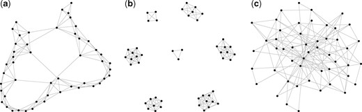
The network topologies of band, block and scale-free graph in simulations. (a) Band, (b) block and (c) scale-free

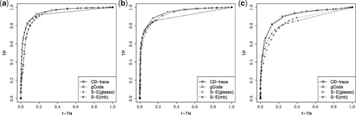
We used CD-trace loss, S-E(mb), S-E(glasso) and gCoda to recover the network for each simulated dataset. The true positive rate and true negative rate were evaluated at different tuning parameters and used to generate the ROC curve. We ran the simulation 100 times for each sample size and graph structure, and then compute the average area under the ROC curve (AUC).

The mean and standard deviation of AUC values for different sample sizes and graph structures are presented in Table 1 and Figure 3. CD-trace achieves higher AUC and lower standard deviation in most cases, implicating that CD-trace is more accurate and stable in network recovery. In band graph, the performance of the four methods is comparable when the sample is relatively small (n = 100), while CD-trace and S-E(mb) performs better with higher AUC and smaller variance when the sample is relatively large (n = 500). For block graph, CD-trace achieves higher AUC across all scenarios (n = 100, 200, 500), and the superiority of CD-trace is more significant when the sample size is larger. In scale-free graph, CD-trace and gCoda performs better than S-E(glasso) and S-E(mb) under different sample sizes (n = 100, 200, 500). Although the performance of gCoda is slightly better than CD-trace when the sample size is 100, the performance of CD-trace is comparable to gCoda when the sample size is 200 and 500. Generally speaking, CD-trace and gCoda performs better than S-E(glasso) and S-E(mb) in most scenarios. As Fang et al. (2017) claimed, the key approximate assumption in S-E(glasso) and S-E(mb) strongly depends on the condition number of the precision matrix, which influences their performance in network inference. The performance of CD-trace is comparable to that of gCoda, benefitting from their similar log-normal distribution and sparsity assumptions. CD-trace further assumes the exchangeable condition, which makes the objective function more concise than that of gCoda. Moreover, the objective function of CD-trace is convex, which avoids the non-convex optimization problem in gCoda. The four methods achieve better performance in band graph and block graph than in scale-free graph. This indicates network inference is also influenced by the graph structure. The ROC curve for different sample sizes and graph structures are shown in Figures 4–6. The result of CD-trace is more stable and has larger AUC in most cases. In general, CD-trace performs better in direct interaction network recovery and estimation.

Table 1.

The mean and standard deviation of AUC values for different sample sizes and graph structures

	n=100	n=200	n=500
	Band
CD-trace	0.8787 (0.0152)	0.9477 (0.0085)	0.9844 (0.0024)
gCoda	0.8651 (0.0136)	0.9245 (0.0082)	0.9600 (0.0036)
S-E(glasso)	0.8678 (0.0124)	0.9089 (0.0103)	0.9355 (0.0064)
S-E(mb)	0.8706 (0.0158)	0.9286 (0.0117)	0.9667 (0.0052)
	Block
CD-trace	0.8598 (0.0175)	0.9405 (0.0090)	0.9856 (0.0027)
gCoda	0.8523 (0.0152)	0.9238 (0.0083)	0.9725 (0.0034)
S-E(glasso)	0.8499 (0.0136)	0.8961 (0.0097)	0.9273 (0.0081)
S-E(mb)	0.8362 (0.0148)	0.8982 (0.0115)	0.9415 (0.0074)
	Scale-free
CD-trace	0.8038 (0.0207)	0.9075 (0.0127)	0.9763 (0.0048)
gCoda	0.8156 (0.0214)	0.9081 (0.0122)	0.9710 (0.0043)
S-E(glasso)	0.7701 (0.0194)	0.8490 (0.0133)	0.9104 (0.0101)
S-E(mb)	0.7492 (0.0220)	0.8469 (0.0170)	0.9330 (0.0099)

Note: The values in parenthesis are standard deviations.

Fig. 3.

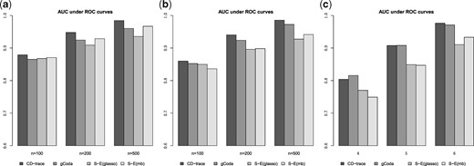
Average area under ROC curve for different sample sizes and graph structures. (a) Band, (b) block and (c) scale-free

Fig. 4.

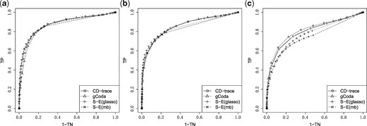
ROC curve for different graph structures with sample sizes n = 100. (a) Band, (b) block and (c) scale-free

Fig. 5.

ROC curve for different graph structures with sample sizes n = 200. (a) Band, (b) block and (c) scale-free

Fig. 6.

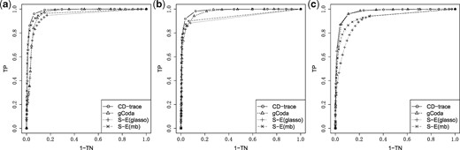
ROC curve for different graph structures with sample sizes n = 500. (a) Band, (b) block and (c) scale-free

3.2 Real data analysis

To validate the performance of CD-trace on recovering the direct interactions from real compositional data, we applied CD-trace, gCoda, S-E(mb) and S-E(glasso) to infer the direct interaction networks of microbes in mouse skin. These mouse skin microbiome data are from a study population of 261 mice (Srinivas et al., 2011), and the samples are divided into three groups according to the health conditions of skin immunizations. The control (Control) group consists of 78 non-immunized samples, and the Healthy group has 119 immunized healthy samples and the epidermolysis bullosa acquisita (EBA) group consists of 64 immunized individuals. We further filtered the data by removing OTUs, the appearance of which did not exceed 60% in samples and by removing samples with more than 60% 0s collected as Fang et al. (2017) did in their analysis. We finally arrived at a dataset with D = 60 OTUs and n = 229 samples (64 Control samples, 112 healthy samples and 53 EBA samples) for evaluation. We added all OTU counts by 0.5 to avoid zero counts and normalized the data to compositional data.

We applied the aforementioned four methods to construct the direct interaction network for each group. Figure 7 represents the difference among the edges recovered by the four methods in each group (Control, Healthy and EBA). The common edges shared by S-E(mb) and S-E(glasso) are more than other combinations, since they are two variants of S-E. A total of 22, 56 and 23 edges were discovered by all four methods for the Control, Healthy and EBA group respectively. Most edges recovered by CD-trace were also verified by the other methods.

Fig. 7.

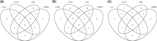
Venn figure of edges recovered by four different methods for each group. (a) Control, (b) healthy and (c) EBA

Since we did not have prior information for the true interaction network among taxons in real data, we compared the consistent reproducibility of the four methods, as suggested by Fang et al. (2017) and Kurtz et al. (2015). To be more specific, we used all data to construct a direct interaction network as our gold standard for each method, and then selected 70% of the samples randomly to estimate the direct interaction network with each method, respectively. The number of edges shared by the sub-sample estimator and the gold standard were measures of the consistent reproducibility. We used the fraction of these common edges in the gold standard as our consistent reproducibility. We repeated this procedure 20 times and summarized the mean consistent reproducibility in Table 2. The consistent reproducibility of CD-trace, gCoda and S-E(glasso) fluctuated around 80%, which is significantly better than S-E(mb). In Control group and EBA group with fewer samples, CD-trace performed slightly better than gCoda and S-E(glasso). For healthy group with more samples, the consistent reproducibility of gCoda and S-E(glasso) was higher than CD-trace. The networks constructed with all data for the three groups are lefted in the Supplementary Figures S1–S3. We also compared the false positive count of the four methods as Fang et al. (2017) did. We used the count of edges inferred by CD-trace, gCoda, S-E(mb) and S-E(glasso) from shuffled data to measure the false positive count, since we expected to find no interaction among species from shuffled data. We generated 20 shuffled datasets to compute the false positive count, and the averaged results are summarized in Table 2. The average false positive count of CD-trace is less than that of the other three methods across all three groups, and the results of S-E(mb) and S-E(glasso) are generally the worst.

Table 2.

Consistent reproducibility and false positive count for CD-trace, gCoda, S-E(mb) and S-E(glasso)

	Consistent reproducibility			False positive count
Group	Control	Healthy	EBA	Control	Healthy	EBA
CD-trace	0.87 (0.04)	0.79 (0.03)	0.85 (0.04)	2.45	2.95	1.70
gCoda	0.85 (0.06)	0.82 (0.04)	0.82 (0.07)	8.50	6.05	5.55
S-E(glasso)	0.86 (0.06)	0.83 (0.05)	0.84 (0.06)	11.45	10.55	12.50
S-E(mb)	0.80 (0.05)	0.75 (0.06)	0.77 (0.06)	12.00	11.10	12.15

Note: The values in parenthesis are standard deviations.

4 Discussion

In this paper, we propose a loss function for compositional data based on D-trace loss, which enabled us to estimate the direct interaction network among microbial communities with observed compositional data. A lasso penalized estimator was proposed and an effective algorithm was developed for numerical estimation. We found that CD-trace performs well in both simulation and real data analysis. The convexity of the CD-trace loss function makes numerical solution more convenient than the non-convex likelihood function in gCoda. Moreover, CD-trace makes use of the bridge between the observed compositional data and the unobserved latent variables, enabling us to estimate the transformed covariance with compositional data directly.

The proposed method is based on compositions instead of counts. The count data of 16S-rRNA genes are usually over-dispersed and highly sparse because of excessive numbers of zeros in count data. We add OTU counts by 0.5 in real applications to avoid zero counts and normalize the data to compositional data, which brings an inflation of $\text{log}(0.5)$ to compositions and it may be oversimplified to assume compositions follow a logistic normal distribution. The excessive numbers of zeros in count data, of course, also contains information for the distribution of compositions and absolute abundances. How to construct models to handle these zeros and make use of information from these zeros needs further study. The same as gCoda and S-E, the computational complexity of CD-trace is $O(p^3)$⁠, since it conducts eigenvalue decomposition in each iteration. Thus, the scalability of CD-trace is comparable with gCoda and S-E. The consistency of the estimator is not guaranteed, which is a common problem of CD-trace, gCoda and S-E. More efforts are needed to establish the theoretical results in relation to the consistency of these estimators.

Funding

This work was supported by the National Key Research and Development Program of China [number 2016YFA0502303]; the National Key Basic Research Project of China [number 2015CB910303]; and the National Natural Science Foundation of China [number 31871342].

Conflict of Interest: none declared.

Author notes

The authors wish it to be known that, in their opinion, Huili Yuan and Shun He authors should be regarded as Joint First Authors.