VIMCO: variational inference for multiple correlated outcomes in genome-wide association studies

Abstract

Motivation

In genome-wide association studies (GWASs) where multiple correlated traits have been measured on participants, a joint analysis strategy, whereby the traits are analyzed jointly, can improve statistical power over a single-trait analysis strategy. There are two questions of interest to be addressed when conducting a joint GWAS analysis with multiple traits. The first question examines whether a genetic loci is significantly associated with any of the traits being tested. The second question focuses on identifying the specific trait(s) that is associated with the genetic loci. Since existing methods primarily focus on the first question, this article seeks to provide a complementary method that addresses the second question.

Results

We propose a novel method, Variational Inference for Multiple Correlated Outcomes (VIMCO) that focuses on identifying the specific trait that is associated with the genetic loci, when performing a joint GWAS analysis of multiple traits, while accounting for correlation among the multiple traits. We performed extensive numerical studies and also applied VIMCO to analyze two datasets. The numerical studies and real data analysis demonstrate that VIMCO improves statistical power over single-trait analysis strategies when the multiple traits are correlated and has comparable performance when the traits are not correlated.

Availability and implementation

The VIMCO software can be downloaded from: https://github.com/XingjieShi/VIMCO.

Supplementary information

Supplementary data are available at Bioinformatics online.

1 Introduction

Genome-wide association studies (GWASs) conducted in the last decade have provided valuable insights into the genetic architecture underlying complex traits. GWAS are generally performed by analyzing individual traits, although multiple related traits are often collected, and in some cases these traits may reflect a common condition (Kim et al., 2009). In a GWAS where multiple traits have been measured on the study individuals, a joint analysis strategy whereby the multiple traits are analyzed jointly, offers improved statistical power when compared with a single-trait analysis strategy, when a genetic variant is associated with one or more correlated phenotypes (Korte et al., 2012; Solovieff et al., 2013). A joint analysis strategy may also be useful when the different phenotypes characterize the same underlying trait.

There are typically two questions of interest to be addressed in a joint GWAS analysis of multiple traits. The first question addresses whether a genetic loci is significantly associated with any of the (correlated) phenotypes being tested. The second question focuses on the identification of the phenotype(s) that is/are associated with the genetic loci. When multiple continuous traits and genotype data are available from the same study individuals, a joint GWAS analysis that addresses the first question can be performed using linear mixed models based methods (Casale, 2016). Examples of linear mixed models based methods include the multi-trait mixed models proposed by Korte et al. (2012) and the multivariate linear mixed models (mvLMM) implemented in the Genome-wide Efficient Mixed Model Association (GEMMA) software (Zhou and Stephens, 2014). A central limitation of these methods is that they cannot address the second question which seeks to identify the tested trait(s) that is/are associated with the genetic loci. Multi-trait variable selection methods based on penalization have also been proposed in this context (Liu et al., 2016; Rothman et al., 2010). However, they cannot be applied to assess associations while controlling the error rate (Carbonetto et al., 2012).

In this article, we propose a novel method, Variational Inference for Multiple Correlated Outcomes (VIMCO), for joint analysis of multiple traits in GWAS that addresses the second question. VIMCO is applicable when individual-level data on multiple traits and genotype are available on the same study individuals. Our proposed method can be viewed as a complementary method to the widely used mvLMM implemented in the GEMMA package, in that it addresses a different but related scientific question and allows one to identify the specific trait that is associated with the genetic loci when performing a joint analysis of multiple traits. A variational Bayesian expectation-maximization (VBEM) algorithm is used to ensure computational efficiency. Through extensive numerical studies and real data analyses, we demonstrate that our proposed approach offers improved statistical power when compared with existing single-trait analysis strategies. The remainder of this article is organized as follows. In Section 2, we describe the model and algorithm that VIMCO uses to perform joint analysis of multiple traits. We then illustrate the performance of VIMCO using numerical simulations and real data analyses in Section 3 and conclude with a discussion in Section 4.

2 Variational inference for multiple correlated outcome

2.1 Model

In this section, we describe the notation and model used for joint modeling of multiple traits in a GWAS using VIMCO. Consider K continuous phenotypes/traits, $Y_1,\dots ,Y_K$⁠, that are measured on N individuals, where Y_k is a N × 1 vector for $k=1,\dots ,K$⁠. Assume that the genome-wide genotype data consists of p SNPs given by, $X_1,\dots ,X_p$where X_j is a N × 1 vector for $j=1,\dots ,p$⁠. Denote $\mathbf{X}=[X_1,\dots ,X_p]\in {ℝ}^{N\times p}$and $\mathbf{Y}=[Y_1,\dots ,Y_K]\in {ℝ}^{N\times K}$⁠. Without loss of generality, we assume that both the phenotypes and genotypes have been centered. We consider the following multivariate linear model:

$$\mathbf{Y}=\mathbf{X}\mathbf{B}+\mathbf{E},$$

(1)

where $\mathbf{B}={[{\beta }_1,\dots ,{\beta }_p]}^{\top }\in {ℝ}^{p\times K},\hspace{0.17em}{\beta }_j={({\beta }_{j1},\dots ,{\beta }_{\mathit{jK}})}^{\top },\hspace{0.17em}j=1,\dots ,p$⁠, and $\mathbf{E}={[e_1^{\top },\dots ,e_N^{\top }]}^{\top }\in {ℝ}^{N\times K}$⁠. We assume that $e_n\sim \mathcal{N}(0,{\Theta }^{-1})$⁠, where Θ is the precision matrix of $\mathbf{E}$ with dimensionality K × K for individuals $n=1,\dots ,N$⁠. The entries in Θ are denoted by ${\theta }_{\mathit{st}},s,t=1,\dots ,K$⁠. Under this model, the correlation in the traits (conditional on the genotypes) is modeled by the off-diagonal terms in ${\Theta }^{-1}$⁠.

We are interested in identifying genetic variants that are associated with one or more traits, which corresponds to the identification of nonzero entries in the matrix $\mathbf{B}$⁠. We consider a spike-slab prior for $\mathbf{B}$and parameterize $\mathbf{B}$as a product of latent variables. Specifically, we assume that ${\beta }_j={\gamma }_j°{\tilde{\beta }}_j={({\gamma }_{j1}{\tilde{\beta }}_{j1},\dots ,{\gamma }_{\mathit{jK}}{\tilde{\beta }}_{\mathit{jK}})}^{\top }$⁠, where $°$denotes the element-wise product and

$${\tilde{\beta }}_{\mathit{jk}}\sim \mathcal{N}(0,{\sigma }_{{\beta }_k}^2), {\gamma }_{\mathit{jk}}\sim a_k^{{\gamma }_{\mathit{jk}}}{(1-a_k)}^{1-{\gamma }_{\mathit{jk}}}.$$

Let $\Phi =\{a_1,\dots ,a_K,{\sigma }_{{\beta }_1}^2,\dots ,{\sigma }_{{\beta }_K}^2,\Theta \}$be the collection of (unknown) model parameters. Accordingly, our probabilistic model can be reparameterized as:

$$\mathrm{Pr}(\mathbf{Y},\tilde{\beta },\gamma |\mathbf{X};\Phi )=\mathrm{Pr}(\mathbf{Y}|\mathbf{X},\tilde{\beta },\gamma ;\Phi )\mathrm{Pr}(\tilde{\beta },\gamma |\mathbf{X};\Phi )$$

$$=\prod _{n=1}^N\mathcal{N}\left(\sum _{j=1}^p{X}_{\mathit{nj}}\left({\gamma }_j○{\tilde{\beta }}_j\right),{\Theta }^{-1}\right)\prod _{j=1}^p\prod _{k=1}^K\left[a_k^{{\gamma }_{\mathit{jk}}}{(1-a_k)}^{1-{\gamma }_{\mathit{jk}}}\mathcal{N}(0,{\sigma }_{{\beta }_k}^2)\right].$$

With this reparameterization, to identify genetic variants that are associated with one or more traits, we need to compute the posterior distribution of the latent variables $(\tilde{\beta },\gamma )$⁠:

$$\mathrm{Pr}(\tilde{\beta },\gamma |\mathbf{Y},\mathbf{X};\Phi )=\frac{\mathrm{Pr}(\mathbf{Y},\tilde{\beta },\gamma |\mathbf{X};\Phi )}{\mathrm{Pr}(\mathbf{Y}|\mathbf{X};\Phi )}$$

$$=\frac{\mathrm{Pr}(\mathbf{Y},\tilde{\beta },\gamma |\mathbf{X};\Phi )}{{\sum }_{\gamma }{\int }_{\tilde{\beta }}\mathrm{Pr}(\mathbf{Y},\tilde{\beta },\gamma |\mathbf{X};\Phi )d\tilde{\beta }}.$$

(2)

We note that VIMCO is an empirical Bayesian approach where the parameters in the Spike-Slab and Normal priors are estimated from the data, i.e. it does not require specification of hyperparameters.

2.2 VBEM algorithm

In this section, we describe the algorithm used for computation of the model parameters and the posterior distribution of the latent variables $(\tilde{\beta },\gamma )$in VIMCO. Exact computation of the posterior distribution (2) is computationally intensive due to the denominator which requires marginalizing over the latent variables $(\tilde{\beta },\gamma )$⁠. To overcome this computational intractability, we derive a computationally efficient VBEM algorithm (Bishop, 2006) to obtain an approximation for the posterior distribution (2). The key idea of the VBEM algorithm is to approximate our computationally intractable posterior distribution (2), with an approximating distribution, which is computationally tractable. The VBEM algorithm proceeds by specifying a family of (variational) distributions, which are parameterized by variational parameters, and choosing the optimal approximating distribution from this family by minimizing the KL divergence between the approximating distributions and our true posterior distribution (2) (Blei et al., 2017). The KL divergence can be viewed as a measure of how different the approximating distribution is from our true posterior distribution (2). The optimal variational distribution is then used as an approximation for the true posterior distribution (2) (Bishop, 2006).

Let $q(\tilde{\beta },\gamma )$be a candidate approximating distribution of our true posterior distribution (2), and let ${\mathrm{E}}_q$denote the expectation taken with respect to $q(\tilde{\beta },\gamma )$⁠. We can decompose the logarithm of the marginal likelihood as

$$\text{log}\hspace{0.17em}p(\mathbf{Y}|\mathbf{X};\Phi )={\mathcal{L}}_q+\text{KL}\left(q\left|\right|\mathrm{Pr}(\tilde{\beta },\gamma |\mathbf{Y},\mathbf{X};\Phi )\right),$$

(3)

where

$$\begin{array}{c}{\mathcal{L}}_q={\mathrm{E}}_q\hspace{0.17em}\text{log}\hspace{0.17em}\left[\frac{\mathrm{Pr}(\mathbf{Y},\tilde{\beta },\gamma |\mathbf{X};\Phi )}{q(\tilde{\beta },\gamma )}\right]\hfill \\ \text{KL}\left(q\left|\right|\mathrm{Pr}(\tilde{\beta },\gamma |\mathbf{Y},\mathbf{X};\Phi )\right)={\mathrm{E}}_q\hspace{0.17em}\text{log}\hspace{0.17em}\left[\frac{q(\tilde{\beta },\gamma )}{\mathrm{Pr}(\tilde{\beta },\gamma |\mathbf{Y},\mathbf{X};\Phi )}\right].\hfill \end{array}$$

Minimizing the KL divergence with respect to the approximating distribution $q(\tilde{\beta },\gamma )$is equivalent to maximizing the evidence lower bound (ELBO) ${\mathcal{L}}_q$⁠. If we allow any possible choice for $q(\tilde{\beta },\gamma )$⁠, then the Kullback-Leibler divergence $\text{KL}\left(q\left|\right|\mathrm{Pr}(\tilde{\beta },\gamma |\mathbf{Y},\mathbf{X};\Phi )\right)$is zero if and only if $q(\tilde{\beta },\gamma )$ is identical to our true posterior distribution (2) almost surely.

In order for the algorithm to be applicable to GWAS data, we require a family of distributions that is sufficiently flexible to accurately approximate the true posterior distribution, while being computationally tractable. We propose using a mean field variational family (Logsdon et al., 2010), which contains distributions $q(\tilde{\beta },\gamma )$of the form

$$q(\tilde{\beta },\gamma )=\prod _j\prod _k\left[q({\tilde{\beta }}_{\mathit{jk}},{\gamma }_{\mathit{jk}})\right].$$

The factorization used in the approximating mean field variational family of distributions makes the VBEM algorithm computationally efficient. The approximation is expected to perform best when the SNPs are independent and in the absence of pleiotropy. If more accurate inferences are needed, more computationally intensive methods may be required.

Given this variational family of distributions, the optimal variational distribution $q^{\ast }({\tilde{\beta }}_{\mathit{jk}},{\gamma }_{\mathit{jk}})$that maximizes the ELBO ${\mathcal{L}}_q$has the form (Bishop, 2006)

$$\text{log}\hspace{0.17em}{q}^{\ast }({\tilde{\beta }}_{\mathit{jk}},{\gamma }_{\mathit{jk}})={\mathrm{E}}_{(j\prime ,k\prime )\ne (j,k)}\left[\text{log}\hspace{0.17em}\mathrm{Pr}(\mathbf{Y},\tilde{\beta },\gamma |\mathbf{X};\Phi )\right]+\text{constant},$$

(4)

where the expectation is taken with respect to all other factors $q({\tilde{\beta }}_{j\prime k\prime },{\gamma }_{j\prime k\prime })$ for $(j\prime ,k\prime )\ne (j,k)$⁠. After some derivations (details are provided in Supplementary Material SA), the optimal variational posterior distribution is given by:

$$\prod _j\prod _k\left[{\alpha }_{\mathit{jk}}^{{\gamma }_{\mathit{jk}}}{(1-{\alpha }_{\mathit{jk}})}^{1-{\gamma }_{\mathit{jk}}}\mathcal{N}{({\mu }_{\mathit{jk}},s_{\mathit{jk}}^2)}^{{\gamma }_{\mathit{jk}}}\mathcal{N}{(0,{\sigma }_{{\beta }_k}^2)}^{1-{\gamma }_{\mathit{jk}}}\right],$$

where the variational parameters (μ_jk, $s_{\mathit{jk}}^2$⁠, α_jk) are given by:

$$\begin{array}{c}{\mu }_{\mathit{jk}}=\frac{{\sum }_t{\theta }_{\mathit{kt}}{X}_j^{\top }\left[Y_t-{\sum }_{j\prime \ne j}{\alpha }_{j\prime t}{\mu }_{j\prime t}{X}_{j\prime }\right]-{\sum }_{t\ne k}{\theta }_{\mathit{kt}}{\alpha }_{\mathit{jt}}{\mu }_{\mathit{jt}}{\Vert X_j\Vert }^2}{{\theta }_{\mathit{kk}}{\Vert X_j\Vert }^2+\frac{1}{{\sigma }_{{\beta }_k}^2}},\hfill \\ s_{\mathit{jk}}^2=\frac{1}{{\theta }_{\mathit{kk}}{\Vert X_j\Vert }^2+\frac{1}{{\sigma }_{{\beta }_k}^2}},\hfill \\ {\alpha }_{\mathit{jk}}\equiv q({\gamma }_{\mathit{jk}}=1)=\frac{1}{1+\text{exp}\hspace{0.17em}\left(-\text{log}\hspace{0.17em}\frac{a_k}{1-a_k}+\frac{1}{2}\left(\frac{{\mu }_{\mathit{jk}}^2}{s_{\mathit{jk}}^2}+\text{log}\hspace{0.17em}\frac{s_{\mathit{jk}}^2}{{\sigma }_{{\beta }_k}^2}\right)\right)}.\hfill \end{array}$$

(5)

To solve for the variational parameters (μ_jk, $s_{\mathit{jk}}^2$⁠, and α_jk) and model parameters (⁠$\Phi$⁠), the VBEM algorithm iterates between two optimization (expectation and maximization) steps until convergence. In the expectation step, we optimize the ELBO ${\mathcal{L}}_q$with respect to the variational parameters (μ_jk, $s_{\mathit{jk}}^2$and α_jk), while holding the model parameters fixed, i.e. compute variational parameters using Equation (5). In the maximization step, we optimize the ELBO ${\mathcal{L}}_q$with respect to the model parameters $\Phi$while holding the variational parameters fixed. With the optimal variational distribution, the ELBO ${\mathcal{L}}_q$can be evaluated in a closed form (details in Supplementary Material SA):

$$\begin{array}{c}{\mathcal{L}}_q=-\frac{1}{2}{\sum }_s{\sum }_t{\theta }_{\mathit{st}}{\left(Y_s-{\sum }_j{X}_j{\alpha }_{\mathit{js}}{\mu }_{\mathit{js}}\right)}^{\top }\left(Y_t-{\sum }_j{X}_j{\alpha }_{\mathit{jt}}{\mu }_{\mathit{jt}}\right)\hfill \\ -\frac{1}{2}{\sum }_s{\theta }_{\mathit{ss}}{\sum }_j{X}_j^{\top }{X}_j[{\alpha }_{\mathit{js}}({\mu }_{\mathit{js}}^2+s_{\mathit{js}}^2)-{\alpha }_{\mathit{js}}^2{\mu }_{\mathit{js}}^2]\\ -{\sum }_j{\sum }_k\left[{\alpha }_{\mathit{jk}}\hspace{0.17em}\text{log}\hspace{0.17em}\frac{{\alpha }_{\mathit{jk}}}{a_k}+(1-{\alpha }_{\mathit{jk}})\hspace{0.17em}\text{log}\hspace{0.17em}\frac{1-{\alpha }_{\mathit{jk}}}{1-a_k}\right]+\frac{N}{2}\text{log}\hspace{0.17em}|\Theta |\hfill \\ +\frac{1}{2}{\sum }_j{\sum }_k{\alpha }_{\mathit{jk}}\left(1+\text{log}\hspace{0.17em}\frac{s_{\mathit{jk}}^2}{{\sigma }_{{\beta }_k}^2}-\frac{{\mu }_{\mathit{jk}}^2+s_{\mathit{jk}}^2}{{\sigma }_{{\beta }_k}^2}\right)+\text{const}.\hfill \end{array}$$

(6)

By taking partial derivatives of the ELBO ${\mathcal{L}}_q$with respect to the model parameters and setting them to zero, we can solve for the model parameters and obtain the update equations for the maximization step:

$$\begin{array}{c}{a}_k=\frac{{\sum }_j{\alpha }_{\mathit{jk}}}{p},\hfill \\ {\sigma }_{{\beta }_k}^2=\frac{{\sum }_j{\alpha }_{\mathit{jk}}({\mu }_{\mathit{jk}}^2+s_{\mathit{jk}}^2)}{{\sum }_j{\alpha }_{\mathit{jk}}},\hfill \\ {({\Theta }^{-1})}_{\mathit{kk}}=\frac{{\Vert Y_k-{\sum }_j{X}_j{\alpha }_{\mathit{jk}}{\mu }_{\mathit{jk}}\Vert }^2}{N}\hfill \\ +\frac{{\sum }_j{\Vert X_j\Vert }^2\left[{\alpha }_{\mathit{jk}}({\mu }_{\mathit{jk}}^2+s_{\mathit{jk}}^2)-{\alpha }_{\mathit{jk}}^2{\mu }_{\mathit{jk}}^2\right]}{N},\hfill \\ {({\Theta }^{-1})}_{\mathit{kt}}=\frac{{\left(Y_k-{\sum }_j{X}_j{\alpha }_{\mathit{jk}}{\mu }_{\mathit{jk}}\right)}^{\top }\left(Y_t-{\sum }_j{X}_j{\alpha }_{\mathit{jt}}{\mu }_{\mathit{jt}}\right)}{N}.\hfill \end{array}$$

(7)

The VBEM algorithm iterates between the expectation (Equation 5) and maximization (Equation 7) steps until convergence. Further details on the VBEM algorithm are provided in Supplementary Material SA.

2.3 Inference

With the estimated variational parameters (μ_jk, $s_{\mathit{jk}}^2$and α_jk) and model parameters (⁠$\Phi$⁠), the posterior probability $\mathrm{Pr}({\gamma }_{\mathit{jk}}=1|\mathbf{Y},\mathbf{X};\Phi )$of whether genetic variant j is associated with trait k can be estimated by ${\widehat{\alpha }}_{\mathit{jk}}$⁠, and the local false discovery rate (lfdr) can be estimated by $1-{\widehat{\alpha }}_{\mathit{jk}}$⁠. Statistical inference can be conducted by identifying SNP-trait associations while controlling the global FDR at a fixed value. Specifically, given a cutoff for the global FDR, the cutoff ξ for the lfdr can be computed from $\text{global} \text{FDR}=\frac{{\sum }_j{\sum }_k{\text{lfdr}}_{\mathit{jk}}\mathbb{I}({\text{lfdr}}_{\mathit{jk}}\le \xi )}{{\sum }_j{\sum }_k\mathbb{I}({\text{lfdr}}_{\mathit{jk}}\le \xi )}$(Newton et al., 2004).

3 Results

3.1 Simulations

We conducted numerical simulations to evaluate the performance of VIMCO. We considered the scenario where we have K = 4 continuous traits and P = 10 000 SNPs that were measured on N = 5000 individuals. For each individual, the p genotypes were simulated by first generating a $p\times 1$multivariate normal distribution assuming auto-regressive (AR) correlation with parameter ρ_x. We then discretized each variable to a trinary variable (0, 1, 2) by assuming Hardy-Weinberg equilibrium and with a minor allele frequency randomly selected from a uniform [0.05, 0.5] distribution. The genotype correlation was varied at ρ_x = 0.2, 0.5, 0.8. To generate the coefficient matrix B, for each trait, we selected 1% of the SNPs to be associated with the trait, where the effect sizes were generated from a standard normal distribution. To allow for pleiotropy where a SNP can be associated with more than one trait, we varied the proportion of causal SNPs that was associated with more than one trait. Let $g=\frac{{\sum }_j\mathbb{I}\left(\sum _k{\gamma }_{\mathit{jk}}\ge 2\right)}{{\sum }_j{\sum }_k{\gamma }_{\mathit{jk}}}$⁠. The expectation of g was varied at 0, 0.15, 0.3, where increasing g reflects increasing pleiotropy. The error matrix $\mathbf{E}$was generated with rows drawn independently from a multivariate normal distribution, with AR correlation parameter ρ_e = 0.2, 0.5, 0.8. A larger value of ρ_e implies a higher correlation between the traits. Each error variance was adjusted according to the pre-specified heritability of h² = 0.3.

To benchmark the performance of VIMCO, we considered both Bayesian [variational inference-based Bayesian variable selection regression (BVSR); Carbonetto et al., 2012] and frequentist [single-trait linear mixed model (sLMM); Zhou and Stephens, 2012] single-trait analysis approaches. Similar to VIMCO, BVSR utilizes a VBEM algorithm, but can only be applied to single traits. sLMM was implemented using the GEMMA software package. For VIMCO and BVSR, we report the statistical power with a global FDR controlled at 0.1. The global FDR for VIMCO and BVSR controls for multiple testing across the multiple traits and SNPs. For sLMM, we report power while controlling for the family wise Type 1 error rate at 0.05, by applying a Bonferroni correction for both the number of SNPs and number of traits tested. We note that this comparison between of VIMCO/BVSR with sLMM may not be on the same footing as they are based on different metrics (FDR versus family wise error rate). The comparison, however, mimics how the methods are commonly used in practice, i.e. by controlling the global FDR for VIMCO and BVSR and by controlling the family wise error rate for sLMM. We compared the power of VIMCO, BVSR and sLMM by considering trait-SNP associations for all traits and SNPs. The power for VIMCO, BVSR and sLMM, for the scenario where the genotypes were strongly correlated (ρ_x = 0.8) and pleiotropy g = 0, is shown in the left panel of Figure 1. When the traits showed moderate (ρ_e = 0.5) or strong correlation (ρ_e = 0.8), VIMCO had higher statistical power than BVSR. When the traits were weakly correlated (ρ_e = 0.2), VIMCO had similar power as BVSR. In all cases, BVSR had higher power than sLMM. We also evaluated the global FDR control for the three approaches. Similar to earlier papers (Brzyski et al., 2017), when evaluating the control of global FDR, the SNPs were evaluated as a cluster of SNPs. i.e. rejections within the same linkage disequilibrium block were grouped and counted as a single rejection. As shown in the middle panel in Figure 1, both VIMCO and BVSR had empirical FDRs that were close to the nominal 0.1 level. sLMM based on controlling for the family wise error rate had well-controlled FDR in this scenario, but the empirical FDR was conservative at lower genotype correlations ρ_x = 0.2 and 0.5 (Supplementary Figs SB1 and SB2), which is not surprising since it controls for the family wise error rate and not the FDR. We also compared the area under the curve (AUC) of VIMCO, BVSR and sLMM (right panel of Fig. 1). The AUC was evaluated by considering trait-SNP associations for all traits and SNPs. The AUC of VIMCO was higher than that of the single-trait approaches (BVSR and sLMM) when the traits showed moderate (ρ_e = 0.5) or strong correlation (ρ_e = 0.8). Simulations with lower genotype correlation ρ_x = 0.2, 0.5 and different levels of pleiotropy g are shown in Supplementary Figures SB1–SB3, and give similar conclusions.

Fig. 1.

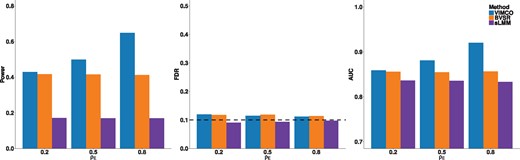
Simulation results for evaluating null hypothesis H_0a, for different ρ_e (increasing levels of ρ_e imply increasing correlation between the traits) and genotype correlation parameter ${\rho }_x=0.8$ Left panel: power of VIMCO, BVSR and sLMM; middle panel: empirical global FDR of VIMCO, BVSR and sLMM; right panel: AUC of VIMCO, BVSR and sLMM

As noted earlier, mvLMM assesses a different but related null hypothesis of whether any of the traits are associated with the genetic variants. Specifically, for the jth SNP, mvLMM evaluates the null hypothesis $H_{0b}:{\beta }_{j1}=\cdots ={\beta }_{\mathit{jK}}=0$⁠, whereas VIMCO evaluates the null hypothesis $H_{0a}:{\beta }_{\mathit{jk}}=0$ for k = 1, …, K traits separately. We evaluated the performance of VIMCO for assessing the null hypothesis H_0b. For evaluating the performance in assessing the null hypothesis H_0b, we performed an ad hoc modification of VIMCO, BVSR and sLMM. In this ad hoc adaptation of VIMCO, BVSR and sLMM, we rejected the null hypothesis H_0b if H_0a is rejected for any of the traits. We examined the power of VIMCO and BVSR while controlling the global FDR at 0.1 For sLMM, we report power while controlling for the family wise Type 1 error rate at 0.05. We also compared the AUC of VIMCO, BVSR, sLMM and mvLMM. Results for the scenario where the genotypes were strongly correlated (ρ_x = 0.8) and the level of pleiotropy g = 0 are shown in Figure 2. Similar to results in evaluating H_0a, VIMCO improves statistical power and has higher AUC when the traits showed moderate or strong correlation. For this ad hoc adaptation of VIMCO and BVSR, the empirical FDR were well-controlled for the settings we considered (middle panel of Fig. 2). We note that evaluating the null hypothesis H_0b is not an intended use of VIMCO, and this ad hoc adaptation of VIMCO was performed in order to provide a comparison with mvLMM. Simulations with different genotype correlation and levels of pleiotropy gave similar conclusions (Supplementary Figs SB4–SB6). To more closely mimic the linkage disequilibrium structure present in real genotype data, we also conducted simulations where we sampled genotypes from chromosome 1 in the NFBC1966 dataset. The linkage disequilibrium structure in real genotype data is likely to be more varied and complex instead of following a simple AR(ρ) structure that we previously examined. We observed slight inflation of the FDR for these simulations (Supplementary Figs SB7 and SB8). A possible reason is that under more complex linkage disequilibrium structures, SNPs correlated to causal SNP(s) may be selected even if they are not in the same linkage disequilibrium block(s), and determining if a selected SNP is representative of a causal SNP becomes more complicated. In cases where tighter control of FDR is required, more computationally accurate methods may be needed.

Fig. 2.

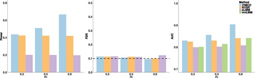
Simulation results for evaluating null hypothesis H_0b, for different ρ_e (increasing levels of ρ_e imply increasing correlation between the traits) and genotype correlation parameter ${\rho }_x=0.8$ Left panel: Power of VIMCO, BVSR and sLMM; middle panel: empirical global FDR of VIMCO, BVSR and sLMM; right panel: AUC of VIMCO, BVSR, sLMM and mvLMM

3.2 Real data analysis

To illustrate the performance of our proposed method VIMCO, we analyzed two datasets. The first dataset is a GWAS of four moderately correlated lipid traits from the Northern Finland Birth Cohort 1966 (NFBC1966). The second dataset is a GWAS of three weakly correlated eye measurements from the Singapore Indian Eye (SINDI) study (Cheng et al., 2013).

3.2.1 NFBC1966

The NFBC1966 dataset consists of 10 metabolic traits and 364 590 SNPs from 5402 individuals (Sabatti et al., 2009). The 10 metabolic traits include fasting lipid levels [total cholesterol (TC), high-density lipoprotein (HDL), low-density lipoprotein (LDL) and triglycerides (TG)], inflammatory marker C-reactive protein, markers of glucose homeostasis (glucose and insulin), body mass index and blood pressure (BP) measurements (systolic and diastolic BP). Quality control of the data was performed using PLINK (Purcell et al., 2007) and GCTA (Yang et al., 2011). Individuals with missing-ness in any of the traits and with genotype missing call-rates > 5% were excluded. We excluded SNPs with minor allele frequency < 1%, missing call-rates > 1%, or failed Hardy-Weinberg equilibrium. After quality control filtering and SNP pruning, 172 412 SNPs from 5123 individuals were available for analysis. We quantile-transformed each trait to a standard normal distribution, obtained the residuals after regressing out the effects of sex, oral contraceptives and pregnancy status, and quantile-transformed the residuals to a standard normal distribution.

We performed analysis on the four lipid traits (TC, LDL, HDL and TG). The pairwise Pearson correlation for the four lipid traits are given in Supplementary Figure SC1. Among the four traits, TC and LDL showed the strongest correlation (corr $=0.88$⁠). Modest correlation was also observed among the following pairs of traits: TG and TC (corr $=0.41$⁠), TG and LDL (corr $=0.33$⁠), TG and HDL (corr $=-0.40$⁠). We applied VIMCO to perform joint analysis of the four traits. For comparison with the results from VIMCO, we also performed single-trait analyses whereby each of the four traits were analyzed separately, using both Bayesian (variational inference-based BVSR; Carbonetto et al., 2012) and frequentist approaches sLMM (Zhou and Stephens, 2012).

For VIMCO and BVSR, we report significant SNP-trait associations at a global FDR of 0.1. The global FDR for VIMCO and BVSR controls for multiple testing across the multiple traits and SNPs. For sLMM, to control for multiple testing across both traits and SNPs, we report P-values for SNP-trait associations with P-value < 1.25 × 10^–8 (we applied a Bonferroni adjustment for the four traits to the commonly used genome-wide significance threshold 5 × 10⁻⁸).

Genomic locations of SNPs identified by VIMCO, BVSR and sLMM are shown in Figure 3. To control the global FDR at 0.1, a SNP has to have a lfdr < 0.73 and < 0.36 for VIMCO and BVSR, respectively (indicated by the horizontal red lines in the plots). VIMCO identified a total of 39 SNP-trait associations, whereas the single-trait analysis strategies BVSR and sLMM identified 34 and 10 SNP-trait associations, respectively. In terms of the total number of unique SNPs identified, VIMCO identified a smaller number of SNPs than BVSR; VIMCO identified 23 SNPs to be associated with at least one trait, while BVSR and sLMM identified 30 and 9 SNPs, respectively. A possible explanation for the lower number of unique SNPs identified by VIMCO is because for traits that showed strong correlation with each other (e.g. TC and LDL), VIMCO identified more SNPs than BVSR and sLMM; while for the remainder traits BVSR and sLMM identified fewer SNPs than VIMCO.

Fig. 3.

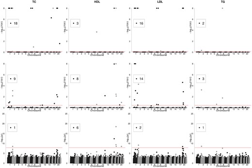
Manhattan plots for the analysis results of VIMCO (first row), BVSR (second row) and sLMM (last row), in the NFBC1966 study. In the first and second row, the horizontal red lines correspond to a global FDR of 0.1. In the last row, the horizontal red line corresponds to a P-value cutoff of 1.25 × 10⁻⁸. The number in the box indicates the number of SNP associations identified for each trait

The lfdrs (VIMCO and BVSR) and P-values (sLMM) of identified SNPs are given in Supplementary Table SC1. For SNPs that were identified by either VIMCO, BVSR or sLMM, we also report their P-values from a mvLMM fitted using the GEMMA package (Zhou and Stephens, 2014). As noted earlier, mvLMM assesses a different but related hypothesis of whether any of the four traits are associated with the genetic variants.

Analysis of the NFBC1966 dataset was conducted on a machine with 3.0 GHz Intel Xeon CPU and 32 G memory. With the BVSR estimates as initial values (1.2 h), it took VIMCO an additional 2.5 h to complete the full variational inference procedure.

3.2.2 Singapore Indian Eye

The SINDI dataset contains three eye measurements: the ratio of BP to intraocular pressure (BP/IOP), central corneal thickness (CCT) and cup-to-disc ratio. These three traits are risk factors for glaucoma (Lavanya et al., 2009). The pairwise correlation for these three traits (Supplementary Fig. SC2) was much weaker than those observed for the lipid traits in the NFBC1966 dataset, with the strongest correlation of 0.16 observed between BP/IOP and CCT. After quality control following previous studies (Cheng et al., 2013) and SNP pruning, 2219 individuals and 257 736 SNPs were available for analysis. Locations of SNPs identified by VIMCO, BVSR and sLMM in the genome are shown in Figure 4. In this dataset where the traits were weakly correlated, the performance for VIMCO was similar as the single-trait approaches. VIMCO and BVSR identified the same two SNPs to be associated with CCT. Among the two associations, rs12447690 was also identified by sLMM (the P-value is 5.5 × 10⁻⁹). This SNP was located in the Zinc-Finger protein (ZNF469) gene, and was previously reported to be associated with CCT (Gao et al., 2016). The lfdrs and P-values of identified SNPs are given in Supplementary Table SC2.

Fig. 4.

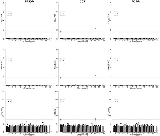
Manhattan plots for the analysis results of VIMCO (first row), BVSR (second row) and sLMM (last row), in the SINDI study. In the first and second row, the horizontal red lines correspond to a global FDR of 0.1. In the last row, the horizontal red line corresponds to a P-value cutoff of 1.67 × 10⁻⁸. The number in the box indicates the number of SNP associations identified for each trait

Analysis of the SINDI dataset used BVSR estimates as initial values (6.8 h), and used an additional 1.2 h to complete the full variational inference procedure.

4 Discussion

In this article, we have proposed a novel method VIMCO that allows an investigator to identify the specific trait that is associated with the genetic loci when performing a joint GWAS analysis of multiple traits. Results from simulations and real data analyses demonstrate that VIMCO improved statistical power when the traits were correlated and had comparable performance when the traits were not correlated, when compared with single-trait analysis strategies. Furthermore, VIMCO utilizes a computationally efficient VBEM algorithm which allows it to handle genome-wide genotype data efficiently. The computational complexity of VIMCO is $O(K^{2}np+K^3)$⁠. For a small number of traits (K) (around 10), the overall computational cost is $O(K^{2}np)$⁠, i.e. the computational time is linear with respect to the sample size n and the number of SNPs p. To demonstrate the run times of VIMCO, Supplementary Figure SB9 shows the average run times for 10 iterations for: (i) $K=4,n\in \{5000,10\hspace{0.17em}000,15\hspace{0.17em}000,20\hspace{0.17em}000\}$ and $p\in \{50\hspace{0.17em}000,100\hspace{0.17em}000,500\hspace{0.17em}000,1\hspace{0.17em}000\hspace{0.17em}000\}$⁠; (ii) p = 500 000, $n\in \{5000,10\hspace{0.17em}000,20\hspace{0.17em}000,40\hspace{0.17em}000\}$and K = 1, …, 5. Computations were conducted on a machine with 3.0 GHz Intel Xeon CPU and 32G memory. For a specific example, for (K, n, p) = (4, 20 000, 1 000 000), the total run time was 94 h. For larger sample sizes, VIMCO can be used if there is sufficient computational memory. For denser genotype data, to ensure computational efficiency, analysis can be performed for each chromosome separately.

VIMCO is, however, not without limitations. First, VIMCO is not applicable when the number of traits analyzed exceeds the number of samples. With increasing interest in performing phenome-wide association studies whereby the number of phenotypes can be larger than the sample size, extending VIMCO to handle larger number of phenotypes is an avenue for future work. Second, VIMCO requires complete genotype and phenotype data for each individual. In practice, missingness can be handled using imputation techniques. Last, VIMCO requires individual-level trait and genotype data to be collected from the same individuals. The development of a method where summary statistics from different individuals can be used for analysis instead of individual-level data is another avenue for future research.

Acknowledgements

The authors are grateful to Minwei Dai for helpful comments and dicussion. The computational work for this article was partially performed on resources of the National Supercomputing Centre, Singapore (https://www.nscc.sg).

Funding

This work was supported in part by [grant numbers 71501089, 11501579 and 71472023] from National Natural Science Foundation of China [grant numbers 22302815, 12316116 and 12301417] from the Hong Kong Research Grant Council [grant R-913-200-098-263 and R-913-200-127-263] from the Duke-NUS and AcRF Tier 2 [MOE2016-T2-2-029, MOE2018-T2-1-046 and MOE2018-T2-2-006] from the Ministry of Education, Singapore.

Conflict of Interest: none declared.