Functional geometry of protein interactomes

Abstract

Motivation

Protein–protein interactions (PPIs) are usually modeled as networks. These networks have extensively been studied using graphlets, small induced subgraphs capturing the local wiring patterns around nodes in networks. They revealed that proteins involved in similar functions tend to be similarly wired. However, such simple models can only represent pairwise relationships and cannot fully capture the higher-order organization of protein interactomes, including protein complexes.

Results

To model the multi-scale organization of these complex biological systems, we utilize simplicial complexes from computational geometry. The question is how to mine these new representations of protein interactomes to reveal additional biological information. To address this, we define simplets, a generalization of graphlets to simplicial complexes. By using simplets, we define a sensitive measure of similarity between simplicial complex representations that allows for clustering them according to their data types better than clustering them by using other state-of-the-art measures, e.g. spectral distance, or facet distribution distance. We model human and baker’s yeast protein interactomes as simplicial complexes that capture PPIs and protein complexes as simplices. On these models, we show that our newly introduced simplet-based methods cluster proteins by function better than the clustering methods that use the standard PPI networks, uncovering the new underlying functional organization of the cell. We demonstrate the existence of the functional geometry in the protein interactome data and the superiority of our simplet-based methods to effectively mine for new biological information hidden in the complexity of the higher-order organization of protein interactomes.

Availability and implementation

Codes and datasets are freely available at http://www0.cs.ucl.ac.uk/staff/natasa/Simplets/.

Supplementary information

Supplementary data are available at Bioinformatics online.

1 Introduction

1.1 Motivation

Genome is the blueprint of a cell. DNA regions called genes are transcribed into messenger RNAs that are translated into proteins. These proteins interact with each other and with other molecules to perform their biological functions. Deciphering the patterns of molecular interactions (also called topology) is fundamental to understanding the functioning of the cell (Ryan et al., 2013). In system biology, molecular interactions are modeled as various molecular interaction networks, in which nodes represent molecules and edges connect molecules that interact in some way. Examples include the well-known protein–protein interaction (PPI) networks in which nodes represent proteins and edges connect proteins that can physically bind.

Because exact comparison between networks has long been known to be computationally intractable (Cook, 1971), the topological analyses of biological networks use approximate comparisons (heuristics), commonly called network properties, such as the degree distribution, to approximately say whether the structures of networks are similar (Newman, 2010). Advanced network properties that utilize graphlets (small induced subgraphs) (Pržulj et al., 2004) have been successfully used to mine biological network datasets. Graphlet-based properties include measures of topological similarities between nodes and between networks (Pržulj et al., 2004, 2007; Yaveroğlu et al., 2014), as well as between protein 3D structures represented by networks (Malod-Dognin and Pržulj, 2014; Faisal et al., 2017). In particular, graphlets have been used to characterize and compare the local wiring patterns around nodes in a PPI network (Milenković and Pržulj, 2008), which revealed that molecules involved in similar functions tend to be similarly wired (Davis et al., 2015). These topological similarities between nodes have also been used to guide the node mapping process of network alignment methods (Kuchaiev et al., 2010; Kuchaiev and Pržulj, 2011; Malod-Dognin and Pržulj, 2015; Vijayan et al., 2015), which allowed for transferring of biological annotation between nodes in different networks of well-studied species to less studied ones.

Despite significant progress, these simple network (also called graph) models of molecular interaction data can only represent pairwise relationships and cannot fully capture the higher organization of molecular interactions, such as protein complexes and biological pathways (Estrada and Rodriguez-Velazquez, 2005). Hence, we need to model these data by using new mathematical formalisms capable of capturing their multi-scale organization. Furthermore, we need to design new algorithms capable of extracting new biological information hidden in the wiring patterns of the molecular interaction data modeled by using these mathematical formalisms. This paper addresses these issues.

1.2 Simplicial complexes basics

A candidate model for capturing higher-order molecular organization is a simplicial complex (Munkres, 1984). A simplicial complex is a set of simplices, where a 0D simplex is a node, a 1D simplex is an edge, a 2D simplex is a triangle, a 3D simplex is a tetrahedron and their n-dimensional counterparts (illustrated in Fig. 1). The dimension of a simplicial complex is the largest dimension of its simplices.

Fig. 1.

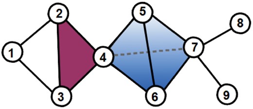
Illustration of a 3D simplicial complex. In the presented simplicial complex, nodes 1, 2 and 3 are only connected by 1D simplices (edges, in black). Nodes 2, 3 and 4 are connected by a 2D simplex (triangle, in magenta). Nodes 4, 5, 6 and 7 are connected by a 3D simplex (tetrahedron, in blue)

The $(n-1)$-dimensional sub-simplices of an n-dimensional simplex are called its faces (e.g. a triangle has three faces, the three edges). A simplicial complex, K, is required to satisfy two conditions:

• For any simplex $\delta \in K$⁠, any face $\delta \prime$ of δ is also in K.

• For any two simplices, ${\delta }_1,{\delta }_2\in K,\hspace{0.17em}{\delta }_1\cap {\delta }_2$ is either $\varnothing$ or a face of both δ₁ and δ₂.

In a simplicial complex, a facet is a simplex that is not a face of any higher-dimensional simplex. Because of this property, a simplicial complex can be summarized by its set of facets.

Note that a network is a 1D simplicial complex and thus, our proposed methodology is directly applicable to both traditional networks and the higher-dimensional simplicial complexes.

While simple network statistics, such as degrees, shortest paths and centralities, have been generalized to simplicial complexes (Estrada and Ross, 2018), the lack of more advanced statistics capturing the geometry of simplicial complexes limits their usage in practical applications.

1.3 Contributions

To comprehensively capture the multi-scale organization of complex molecular networks, we propose to model them by using simplicial complexes. To extract the information hidden in the geometric patterns of these models, we generalize graphlets to simplicial complexes, which we call simplets. Our simplets extend the applicability of graphlets to high-dimensional simplicial complexes. When applied to 1D simplicial complexes, i.e. networks, they are identical to graphlets. On large scale real-world and synthetic simplicial complexes, we show that simplets can be used to define a sensitive measure of geometric similarity between simplicial complexes. Then, on simplicial complexes capturing the protein interactomes of human and yeast, we show that simplets can be used to relate the local geometry around proteins in simplicial complexes with their biological functions. Comparison between 1D PPI networks and the higher-dimensional simplicial complex representations of the interactomes formed by protein interactions and protein complexes shows that higher-order modeling enabled by simplicial complexes allows for capturing more biological information, which can efficiently be mined with our proposed simplets.

2 Materials and methods

2.1 Datasets and their simplicial complex representations

2.1.1 Yeast and human protein interactomes

From BioGRID (v. 3.4.156)(Chatr-Aryamontri et al., 2017), we collected the experimentally validated PPI networks of human (Homo sapiens) and of yeast (Saccharomyces cerevisiae). From CORUM (Ruepp et al., 2010), we collected (on 2 July, 2017) the experimentally validated protein complexes of human, and from CYC2008 (v.2.0) (Pu et al., 2009) the experimentally validated protein complexes of yeast. We consider two different models of an organism’s interactome.

The 1D PPI network: it is the usual PPI network, in which proteins (nodes) are connected by an edge if they can physically bind. Recall that a network is a 1D simplicial complexes on which our new simplet methodologies can be applied and are equivalent to the standard graphlet methodologies.

The higher-dimensional PPI Complex: starting from the PPI network, we additionally connect by simplices all the proteins that belong to common complexes. That is, the proteins belonging to a k-protein complex are connected by a $(k-1)$ dimensional simplex.

For human, the PPI network has 16 100 nodes and 21 319 edges. When unifying the lower dimensional PPI data and the higher-order protein complex data as described above, the resulting PPI Complex is a 140D simplicial complex having 16 140 nodes (with 40 proteins being part of proteins complexes but not having any reported PPI) and 205 192 facets. For yeast, the PPI network has 5842 nodes and 80 900 edges. When unifying the lower dimensional PPI data and the higher-order protein complex data as described above, the resulting PPI Complex is a 80D simplicial complex having 5842 nodes and 76 790 facets.

2.1.2 Other real-world datasets

We collected real-world higher-dimensional datasets from biology and beyond.

• A total of 1569 simplicial complexes of protein 3D structures: Proteins are linear arrangements of amino acids that in the aqueous environment of the cell fold and acquire specific 3D shapes called tertiary structures. We collected from Astral-40 (SCOPe v.2.06) (Fox et al., 2014) the 3D structures of 1569 protein domains that are at-least 100 amino acid long. Each protein domain is modeled as a simplicial complex in which simplices connect together all the amino acids (nodes) that are <7.5 Å apart (as measured by the distances between their α-carbons).

• A total of 132 simplicial complexes of publication authorships: From the pre-print repository arXiv, we collected all the scientific publications in the ‘computer science’ category over 11 years from 2007 to 2017. For each month, we model the scientific collaborations as a simplicial complex in which simplices are formed by all scientists (nodes) that co-authored a scientific publication.

• A total of 60 simplicial complexes of genes’ biological annotations: We collected pathway annotations from Reactome database (v.63) (Fabregat et al., 2018), as well as the experimentally validated Gene Ontology (GO)(Ashburner et al., 2000) annotations from NCBI’s entrez web-server (collected in February 2018). For GO, we consider biological process, molecular function and cellular component annotations separately. For each annotation set, we model the functional annotations of the genes of a given species as a simplicial complex in which simplices are formed by all genes (nodes) that have a common annotation term (restricted to terms annotating up-to 50 genes for computational complexity issues). We only considered simplicial complexes having more than 100 nodes. Following this procedure, we generated 18 pathway simplicial complexes, 13 biological process simplicial complexes, 14 molecular function simplicial complexes and 15 cellular component simplicial complexes.

• A total of 14 simplicial complexes of PPIs: We collected the experimentally validated PPIs from BioGRID database (v. 3.4.156)(Chatr-Aryamontri et al., 2017). These PPIs are first modeled as networks in which proteins (nodes) are connected by edges if they can interact. The corresponding networks are converted into so-called clique complexes, by creating a simplex between all nodes belonging to a maximal clique in the network.

2.1.3 Random simplicial complexes

To test our methods, we considered randomly generated simplicial complexes, which we generate according to ten random models (detailed in Supplementary Material, Section 1).

The first five models are based on randomly generated graphs, which are converted into so-called clique complexes, in which simplices connect nodes that belong to a clique in the graph.

• A random clique complex is the clique complex of an Erdös–Rènyi random graph (Erdös and Rényi, 1959).

• A Vietoris–Rips complex (Hausmann et al., 1995) is the clique complex of a geometric random graph (Penrose, 2003).

• A scale-free complex is the clique complex of a Barabàsi–Albert scale-free graph (Barabási and Albert, 1999).

• A Watts–Strogatz complex is the clique complex of a small-world graph (Watts and Strogatz, 1998).

• An nPSO complex is the clique complex of a non-uniform Popularity Similarity Optimization graph (Muscoloni and Cannistraci, 2018).

The five other models are extensions of the Linial–Meshulam model (Linial and Meshulam, 2006; Meshulam and Wallach, 2009), which originally consists in randomly connecting nodes with kD facets. We extended this model to randomly connect nodes with facets while following the facet distribution of an input simplicial complex. In this way, we can create Linial–Meshulam variant of the five clique complex-based models presented above.

• A Linial–Meshulam random clique complex is a Linial–Meshulam complex that follows the facet distribution of an input random clique complex.

• A Linial–Meshulam Vietoris–Rips complex is a Linial–Meshulam complex that follows the facet distribution of an input Vietoris–Rips complex.

• A Linial–Meshulam scale-free complex is a Linial–Meshulam complex that follows the facet distribution of an input scale-free complex.

• A Linial–Meshulam Watts–Strogatz complex is a Linial–Meshulam complex that follows the facet distribution of an input Watts–Strogatz complex.

• A Linial–Meshulam nPSO complex is a Linial–Meshulam complex that follows the facet distribution of an input nPSO complex.

For each model we choose three node sizes, 1000, 2000 and 3000 nodes, and three edge densities, 0.5, 0.75 and 1%. We generated 25 random simplicial complexes for each model and each of these node sizes and edge densities. Hence, in total, we generated $10\times 3\times 3\times 25=$ 2250 random simplicial complexes. We chose these node sizes and edge densities to roughly mimic the sizes and densities of real-world data detailed above.

2.2 Capturing the local geometry around nodes in a simplicial complex with simplets

We define simplets as small, connected, non-isomorphic, induced simplicial complexes of a larger simplicial complex. Figure 2 shows the eighteen 2- to 4-node simplets (denoted by S₁–S₁₈). Within each simplet, because of symmetries, some nodes can have identical geometries. Analogous to automorphism orbits in graphlets (Pržulj, 2007), we say that such nodes belong to a common simplet orbit group, or orbit for brevity. Figure 2 shows the 32 orbits of the 2- to 4-node simplets (denoted from 1 to 32). Similar to graphlets, we use simplets to generalize the notion of the node degree: the ith simplet degree of node v, denoted by v_i, is the number of times node v touches a simplet at orbit i.

Fig. 2.

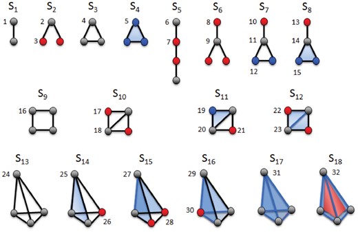
Illustration of 2- to 4-nodes simplets. The eighteen 2- to 4-nodes simplets are denoted by S₁–S₁₈. Within each simplet, geometrically interchangeable nodes, belonging to the same orbit, have the same color. These simplets have 32 different orbits, denoted from 1 to 32. Note that simplets S₄, S₈, S₁₁ and S₁₄ have only one 2D face (triangle, in blue), while S₁₂ and S₁₅ have two triangles, S₁₆ has 3 triangles and S₁₇ has four triangles. S₁₈ has four triangles and one 3D face (tetrahedron, in red)

We define the simplet degree vector (SDV) of a node as the 32D vector containing the simplet degrees of the node in the simplicial complex as its coordinates. Hence, the SDV of a node describes the local geometry around the node in the simplicial complex and comparing the SDVs of two nodes provides a measure of local geometric similarity between them.

We define the SDV similarity between two nodes as an extension of the graphlet degree similarity (Milenković and Pržulj, 2008). It is computed as follows. The distance, $D_i(u,v)$⁠, between the ith simplet orbits of nodes u and v is defined as:

$$D_i(u,v)=w_i\times \frac{|\log (u_i+1)-\log (v_i+1)|}{\log (\max \{u_i,v_i\}+2)},$$

(1)

where w_i is the weight of orbit i that accounts for dependencies between orbits. Weight, w_i, is computed as $w_i=1-\frac{\hspace{0.17em}\text{log}(o_i)}{\hspace{0.17em}\text{log}(32)}$⁠, where o_i is the number of orbits that orbit i depends on, including itself. For instance, the count of orbit 2 (the middle of a three node path) of a node depends on its count of orbit 0 (i.e. its node degree) and on itself, so $o_2=2$⁠. For orbit 9, o₉ = 3, since it is affected by orbits 0, 2 and itself. The values of o_i for all 2- to 4-nodes simplet orbits are listed in Supplementary Table S1. Finally, the SDV similarity, S(u, v), between nodes u and v is defined as:

$$S(u,v)=1-\frac{\sum _{i|(u_i\ne 0) \text{or} (v_i\ne 0)}{D}_i(u,v)}{\sum _{i|(u_i\ne 0) \text{or} (v_i\ne 0)}{w}_i}.$$

(2)

S(u, v) is in (0, 1), where similarity 1 means that the SDVs of nodes u and v are identical.

2.3 Capturing the global geometry of a simplicial complex with simplets

To the best of our knowledge, researchers from computational geometry have not considered the problem of comparing two simplicial complexes. However, the comparison of biological networks is a foundational problem of system biology. Instead, computational geometry focuses on the comparison of two spaces, each represented by a collection of simplicial complexes (e.g. Collins et al., 2004). Thus, we build upon network analysis and extend graphlet and non-graphlet-based network distance measures to directly compare simplicial complexes as follows.

2.3.1 SCD

Simplets are like Lego pieces that assemble with each other to build larger simplicial complexes. We exploit this property to summarize the complex structures of simplicial complexes and to compare them, by generalizing Graphlet Correlation Distance (Yaveroğlu et al., 2014), which is a sensitive measure of topological similarity between networks.

Analogous to graphlets, the statistics of different simplet orbits are not independent of each other. The reason behind this is the fact that smaller simplets are induced sub-simplicial complexes of larger simplets. In Supplementary Material, Section 2, we present the four, non-redundant dependency equations between the simplet degrees of a given node u that we used to assess the correctness of our exhaustive simplet counter.

In addition to these redundancies there also exist dependencies between simplets, which are dataset dependent. We use these dataset dependent simplet orbit dependencies to characterize the global geometry of simplicial complexes. We capture the dependencies between simplet orbits by the simplicial complex’s Simplet Correlation Matrix (SCM), which we define as follows. We construct a matrix whose rows are the SDVs of all nodes of the simplicial complex. We calculate the Spearman’s correlation between each two pairs of columns in the resulting matrix, i.e. correlations between the orbits over all nodes of the simplicial complex. We present these correlations in a 32 × 32 dimensional SCM: it is symmetric and contains Spearman’s correlation values in [−1, 1] range. As presented in Supplementary Figure S1, the SCMs of simplicial complexes from different random simplicial complex models are indeed very different. We exploit these differences in SCMs to compare simplicial complexes.

We define the simplet correlation distance (SCD) to measure the distance between two simplicial complexes, K₁ and K₂, by the Euclidean distance between the upper-triangles of their SCMs:

$$\mathit{SCD}(K_1,K_2)=\sqrt{\sum _{i=1}^{32}\sum _{j=i+1}^{32}{(\mathit{SC}{M}_{K_1}[i][j]-\mathit{SC}{M}_{K_2}[i][j])}^2},$$

(3)

where $\mathit{SC}{M}_{K_1}[i][j]$ is the $(i,j)\text{th}$ entry in the SCM of K₁ (similar for K₂). The ability of SCD to group together simplicial complexes according to their underlying models is demonstrated in Section 3.1.

2.3.2 Facet distribution distance

In analogy to degree distribution and graphlet degree distribution (Pržulj, 2007), we define the measure of connectivity of a k-dimensional simplicial complex, K, as the distribution of its facets, d_K: it is a kD facet distribution vector whose ith entry is the percentage of the facets in K having dimension i. The facet distribution distance (FDD) measures the distance between two simplicial complexes, K₁ and K₂, by the Euclidean distance between their facet distribution vectors, $d_{K_1}$ and $d_{K_2}$⁠:

$$\mathit{FDD}(K_1,K_2)=\sqrt{\sum _i{(d_{K_1}[i]-d_{K_2}[i])}^2}.$$

(4)

2.3.3 Spectral distance

Spectral theory captures the topology of networks and simplicial complexes by using the eigen-values and eigen-vectors of matrices representing them, such as the adjacency matrix, or Laplacian matrix (Wilson and Zhu, 2008). Let H be the incidence matrix of a simplicial complex, K, having n nodes and f facets: H is a n × f matrix in which entry $H[i][j]=1$ if node i is in facet j, and 0 otherwise. The corresponding degree matrix, D, is a n × n diagonal matrix in which entry $D[i][i]$ is the number of facets containing node i. The adjacency matrix, A, of a simplicial complex is: $A=H{H}^T-D$⁠, where H^T is the transpose of H (Zhou et al., 2006). The corresponding Laplacian matrix, L, is: $L=\frac{1}{2}{D}^{-1/2}A{D}^{-1/2}$⁠.

The eigen-decomposition of the Laplacian matrix, L, of simplicial complex, K, is $L=\varphi {\lambda }_K{\varphi }^T$⁠, where ${\lambda }_K=\mathit{diag}({\lambda }_K^1,{\lambda }_K^2,\dots ,{\lambda }_K^n)$ is the diagonal matrix with the ordered eigen-values, ${\lambda }_K^i$ as elements and $\varphi =({\varphi }_1|{\varphi }_2|\dots |{\varphi }_n)$ is the matrix with the ordered eigen-vectors as columns. The spectrum of simplicial complex, K, is the set of its eigen-values $S_K=\{{\lambda }_K^1,{\lambda }_K^2,\dots ,{\lambda }_K^n\}$⁠, which are reordered so that ${\lambda }_K^1\ge {\lambda }_K^2\ge \dots \ge {\lambda }_K^n$⁠.

We define the spectral distance (SD) between two simplicial complexes, K₁ and K₂, as the Euclidean distance between their spectra (Wilson and Zhu, 2008):

$$\mathit{SD}(K_1,K_2)=\sqrt{\sum _i{({\lambda }_{K_1}^i-{\lambda }_{K_2}^i)}^2}.$$

(5)

When the two spectra are of different sizes, 0 valued eigen-values are added at the end of the smaller spectrum.

3 Results and discussion

3.1 Comparing simplicial complexes

A sensitive measure of simplicial complex similarity should find smaller distances between simplicial complexes from the same model than between simplicial complexes from different models.

We visually assess if our SCD (presented in Section 2.3.1) has this property by embedding simplicial complexes as points in 3D space, so that the Euclidean distances between the points in the 3D space best approximate the SCD distances between the corresponding simplicial complexes. We do by using multi-dimensional scaling (MDS) (Borg and Groenen, 2005). As presented in Figure 3, when using the 2250 model simplicial complexes described in Section 2.1.2, we observe that simplicial complexes from the same models are grouped together (i.e. they have small SCD distances), while simplicial complexes from different models are well separated (i.e. they have larger SCD distances).

Fig. 3.

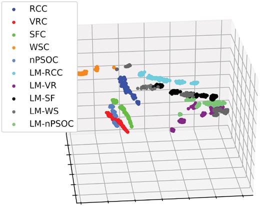
Illustration of MDS-based embedding of simplicial complexes from 10 random models. The randomly generated simplicial complexes (color-coded) are embedded into 3D space according to their pairwise SCD distances using MDS. The 10 models and simplicial complex sizes and densities are described in Section 2.1.2. As described in Section 2.1.2, 25 simplicial complexes are generated for each model and each of its sizes and densities. The grouping of the same colored nodes correspond to simplicial complexes from the same model, which may be of different sizes and densities

We apply SCD and of the two other distances measures described in Section 2.3 on the 2250 model simplicial complexes described in Section 2.1.2, which results for each distance measure between all 2 530 125 pairs of these 2250 simplicial complexes. We formally assess the ability of the distance measure to group together the simplicial complexes from the same model by using the standard precision-recall and receiver operating characteristic (ROC) curves analyses. The resulting precision-recall and ROC curves, which are presented in Supplementary Figures S2 and S3, confirm our visual illustration of the ability of SCD to classify simplicial complexes. We find that SCD achieves the highest classification performance with average precision (AP) of 97.58% and an area under the ROC curve (AUC) of 84.93%. It is followed by the FDD (AP of 96.00% and AUC of 78.73%) and by the SD (AP of 91.42% and AUC of 60.52%).

We further validate our methodology by assessing its ability to correctly group our 1775 real-world simplicial complexes. We calculate the distances between all pairs of the 1775 real-world simplicial complexes, which results in distances between $\left(\begin{array}{c}1775\\ 2\end{array}\right)$ = 1 574 425 pairs for each of the three distance measures presented in Section 2.3. As illustrated in Figure 4, when the real-world simplicial complexes are embedded into 3D space based on their SCD distances by using MDS, the simplicial complexes from the same data type group well together. Out of the four types of real-world simplicial complexes, the ones capturing PPIs are less well clustered, i.e. these simplicial complexes are more variable than the other ones. This could be due to the incompleteness and noisiness of PPI data (Sprinzak et al., 2003), as well as to evolutionary differences in the wiring patterns of the species’ interactomes, as our dataset includes diverse species, such as Arabidopsis thaliana (a plant), H.sapiens (a mammal) and S.cerevisiae (a fungus).

Fig. 4.

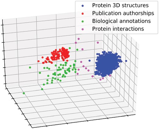
Illustration of MDS-based embedding of real-world simplicial complexes based on their SCDs. The real-world simplicial complexes (color-coded) are embedded into 3D space according to their pairwise SCD distances using MDS

Nevertheless, the precision-recall curves presented in Supplementary Figures S4 and S5 show that SCD achieves the highest classification performances (AP of 98.72% and AUC of 99.58%), followed by SD (AP of 94.93% and AUC of 98.64%) and by FDD (AP of 76.10% and AUC of 93.11%). Taken altogether, our results demonstrate that SCD is a very sensitive measure of simplicial complex similarity.

3.2 Uncovering biological information from PPI Complexes

In the experiments presented above, we measured the ability of simplets to capture global geometric features of simplicial complexes. In this section, we focus on the local geometry around nodes in simplicial complexes. We assess if the local geometries of proteins in PPI Complexes (which we capture with SDVs, see Section 2.2) relate to their functional annotations using two different methodologies: clustering and enrichment analysis of the resulting clusters, and canonical correlation analysis (CCA).

3.2.1 Clustering and enrichment analysis

In system biology, studies, such as Davis et al. (2015) have shown that proteins having similar local wiring patterns in PPI networks tend to have similar biological functions. This suggests that specific protein functions are performed through specific patterns of PPIs, and that the biological functions of unannotated proteins can be predicted from their wiring patterns in the PPI network (Milenković and Pržulj, 2008). This may be explained by evolutionary processes, as genomes are believed to have evolved through gene (and sometimes entire genome) duplication and mutation events. Genes with the same origin have similar sequences and their protein product structures, resulting in similarities in the wiring patterns of their PPIs.

Here, we investigate if a similar property holds in our higher-dimensional representations of interactomes, i.e. if proteins with similar local geometries (as captured by simplets) also tend to have similar biological functions. To this aim, we cluster proteins having similar local geometries (i.e. having similar SVDs) and assess if the obtained clusters are functionally enriched in biological functions as follows. For both human and yeast, we computed the simplet degree similarity of the proteins in each of the two models of their interactomes (PPI network and PPI Complex, see Section 2.1.1). We used these pairwise similarities as input for spectral clustering (Von Luxburg, 2007), which performs k-means clustering on the eigen-vectors of the matrix encoding the pairwise simplet degree similarities between the nodes. Spectral clustering is favored over traditional k-means as it does not make strong assumptions on the shape of the clusters. While k-means produces clusters corresponding to convex sets, spectral clustering can solve a more general problem such as intertwined spirals (Von Luxburg, 2007). To account for the randomness of the underlying k-means, each clustering experiments is repeated 10 times. As there is no gold-standard way of setting the number of clusters, k, we choose the frequently used rule of thumb (Kodinariya and Makwana, 2013), $k=\sqrt{\frac{n}{2}}$⁠, where n in the number of nodes in the simplicial complex. To further motivate our choice of k, we performed 10 spectral clusterings for each k from 10 to 150 in steps of 10. For each value of k, we measured the consistency of the obtained clusterings by using both their sum of square error and their normalized mutual information scores. We observe that the rule of thumb leads to stable clusterings, as $k=\sqrt{\frac{n}{2}}$ is after the elbows of the two consistency scores. That is, we set k = 90 for human and k = 54 for yeast dataset. For comparison purposes, we also generated for both human and yeast 100 random clusterings having same cluster sizes as the ones obtained by spectral clustering on the PPI Complexes.

Then, we measure the biological coherence of the obtained clustering by the percentage of clusters that are statistically significantly enriched in at-least one GO annotation (Ashburner et al., 2000). To this aim, we collected the experimentally validated GO annotations of genes from NCBI’s entrez web portal (collected on 8 March, 2018). We considered GO biological process (GO-BP), GO molecular function (GO-MF) and GO cellular component annotations separately. A cluster is statistically significantly enriched in a given annotation if the corresponding enrichment P-value is lower than or equal to 5% after Benjamini–Hochberg (Benjamini and Hochberg, 1995) correction for multiple hypothesis testing.

As presented in Figure 5, over all ten runs, for both species and for the three GO annotation types, the biological coherence in terms of enriched clusters is larger for the PPI Complexes than for the PPI networks. On average, 79.5% of the clusters from the PPI Complexes are significantly enriched in GO-BP annotations, versus 50.7% for the clusters from the PPI networks. Similarly, 69.8% of the clusters from the PPI Complexes are significantly enriched in GO-MF annotations, versus 44.8% for the clusters from the PPI networks. Finally, 74.2% of the clusters from the PPI Complexes are significantly enriched in GO-BP annotations, versus 53.1% for the clusters from the PPI networks. These results are all statistically significant (with empirical P-values $\le$1%), as the randomly generated clusters are never observed to be as enriched in biological functions than the clusters obtained from the PPI Complex (the random clusterings have, on average, <1% of their clusters with at least one enriched function).

Fig. 5.

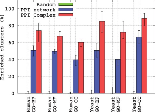
Biological relevance of clusters of genes, as measured by the percentage of clusters having at least one enriched GO annotation. For PPI networks and PPI Complexes, the error bars present minimum, average and maximum enrichment values over 10 runs of spectral clustering, while for Random the error bars present minimum, average and maximum enrichment values over 100 random clustering having same cluster sizes as the ones obtained for PPI Complexes

These results demonstrate that proteins having similar geometries in PPI Complexes, i.e. that form complex interactions in similar ways, indeed tend to have similar biological functions. This may be due to duplications and divergence of the genome regions coding for these molecular machines. Also, our results show that PPI Complex representation captures more biological annotations than simple PPI network representation of these complex data. This illustrates the importance of modeling and wiring of protein interactomes.

3.2.2 Canonical correlation analysis

To quantify the relationships between the local geometry around proteins in simplicial complexes and their biological functions, i.e. to measure how well the simplet degrees of the proteins are predictive of their GO-BP annotations, we adapt the CCA methodologies from Yaveroğlu et al. (2014). The local geometry around n proteins in a simplicial complex is captured in an $n\times 32$ matrix, R, whose entry $R[v][i]$ is the ith simplet degree of node v. Similarly, the biological functions of the proteins are captured in an n × f matrix, A, whose entry $A[v][i]$ is 1 if protein v is annotated by term i, and 0 otherwise. For both matrices, we excluded the genes that do not have any GO-BP annotations. CCA is an iterative process that identifies linear relationships between the 32 simplet degrees and the f GO-BP annotations. First, CCA outputs two weight vectors, called canonical variates, so that the weighted sum of R is maximally correlated with the weighted sum of A. The correlation between the two weighted sums is called their canonical correlation. After finding the first canonical variates, CCA iterates $\min \left\{32,f\right\}$ times to find more weight vectors, such that the resulting canonical variates are not correlated with any of the previous canonical variates. We refer the interested reader to Weenink (2003) for the mathematical aspects of CCA.

As presented in Figure 6 and Supplementary Figure S6, the PPI Complex allows for uncovering a larger number of linear relationships that the PPI network model. This is because only 15 out of the 32 simplets can appear in 1D simplicial complexes, i.e. a PPI network, which corresponds to the fifteen 2- to 4-node graphlets. Hence, CCA can only produce up-to 15 variates for a PPI network and up-to 32 variates for the PPI Complex. Moreover, these linear relationships have higher canonical correlations. This means that by using simplets on the PPI Complexes we can capture more and better quality relationships between local geometry around nodes in simplicial complexes and their biological functions than if we use PPI networks. The same is observed when using GO cellular component and GO-MF annotations (not shown due to space limitations).

Fig. 6.

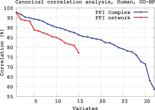
Canonical correlation analysis for human. For a given simplicial complex, canonical correlation produces variates, which are linear combinations of go annotations and linear combinations of simplet degrees that best correlate over the nodes of the simplicial complex. For both models of human interactomes (PPI network and PPI Complex), we plotted for each variate the corresponding correlation value (only statistically significantly correlated variates are presented, with canonical correlation P-value $\le 5\%$⁠)

4 Conclusion

We demonstrate that by the new way of accounting for multi-scale organization of PPI data both through modeling and new algorithms that we propose, we can uncover substantially more biological information than can be obtained by considering only pairwise interactions between proteins in PPI networks. This pioneering observation can further be utilized to predict biological functions of unannotated genes, which is a subject of further research.

We demonstrate the existence of the functional geometry in the PPI data by capturing the higher-order organization of these molecular networks by using simplicial complexes. To mine the geometry of simplicial complexes, we propose simplets, which generalize graphlets to simplicial complexes. On randomly generated and real-world datasets, we define a sensitive measure of global geometrical similarity between simplicial complexes. Also, we propose a higher-dimensional, simplicial complex-based model of a species’ interactome that we call PPI Complex, which combines PPI and protein complex data. On human and yeast interactomes, by using clustering based on our new simplet-based measures of geometric similarity and cluster enrichment analysis, we show that our PPI Complexes are more biologically coherent than PPI networks and that our simplets can efficiently mine PPI Complexes as a new source of biological knowledge. Furthermore, while we focus on simplicial complexes emerging from molecular network organization, our methodology is generic and can be applied to multi-scale datasets from any scientific field, such as the multi-scale network data from physics, social sciences and economy.

Funding

This work was supported by the European Research Council Starting Independent Researcher Grant [278212]; the European Research Council Consolidator Grant [770827]; the Serbian Ministry of Education and Science Project III44006; the Slovenian Research Agency project J1-8155; and the awards to establish the Farr Institute of Health Informatics Research, London, from the Medical Research Council, Arthritis Research UK, British Heart Foundation, Cancer Research UK, Chief Scientist Office, Economic and Social Research Council, Engineering and Physical Sciences Research Council, National Institute for Health Research, National Institute for Social Care and Health Research and Wellcome Trust [grant MR/K006584/1].

Conflict of Interest: none declared.