AuTom-dualx: a toolkit for fully automatic fiducial marker-based alignment of dual-axis tilt series with simultaneous reconstruction

Abstract

Motivation

Dual-axis electron tomography is an important 3 D macro-molecular structure reconstruction technology, which can reduce artifacts and suppress the effect of missing wedge. However, the fully automatic data process for dual-axis electron tomography still remains a challenge due to three difficulties: (i) how to track the mass of fiducial markers automatically; (ii) how to integrate the information from the two different tilt series; and (iii) how to cope with the inconsistency between the two different tilt series.

Results

Here we develop a toolkit for fully automatic alignment of dual-axis electron tomography, with a simultaneous reconstruction procedure. The proposed toolkit and its workflow carries out the following solutions: (i) fully automatic detection and tracking of fiducial markers under large-field datasets; (ii) automatic combination of two different tilt series and global calibration of projection parameters; and (iii) inconsistency correction based on distortion correction parameters and the consequently simultaneous reconstruction. With all of these features, the presented toolkit can achieve accurate alignment and reconstruction simultaneously and conveniently under a single global coordinate system.

Availability and implementation

The toolkit AuTom-dualx (alignment module dualxmauto and reconstruction module $volrec\_mltm$⁠) are accessible for general application at http://ear.ict.ac.cn, and the key source code is freely available under request.

Supplementary information

Supplementary data are available at Bioinformatics online.

1 Introduction

Electron Tomography (ET) has become an indispensable tool for structural biology, in which the three-dimensional density of the ultrastructure is reconstructed from a series of micrographs (tilt series) taken in different orientations (Fernández, 2012; Frank, 2006; Lučić et al., 2013). Most of the tilt series are collected within the tilt angular range $\pm {60}^{°}$ and result in a wedge of missing data, i.e. the ‘missing wedge’ effect, which is one of the main causations of artifacts in reconstruction and the degeneration of resolution. Dual-axis electron tomography (Mastronarde, 1997; Penczek et al., 1995) is an extension to the traditional single-axis technology and can partially compensate for the ‘missing wedge’ issue by having two tilt series taken approximately perpendicular to each other. In recent years, dual-axis tomographic reconstruction has proved its effectiveness in improving resolution (Arslan et al., 2006; Guesdon et al., 2013; Haberfehlner et al., 2014; Sousa et al., 2011).

The most universal workflow for dual-axis tomography is to reconstruct two single-axis tomograms separately and then combine the separately reconstructed tomograms into one single volume (Mastronarde, 1997) (for the convenience of further discussion, we denote this strategy as ‘reconstruction-combination’). Firstly, the specimen taken by dual-axis electron tomography is mostly aimed at cellular analysis and has a relatively large field of view, in which a mass of fiducial markers may exist so that tracking becomes error-prone and time-consuming (Han et al., 2015, 2018; Mastronarde and Held, 2017). Then, merging the two separately reconstructed tomograms requires a mapping matrix. However, solving the mapping matrix related to the two tomograms as well as the following warping correction (Cantele et al., 2007) heavily depends on the intrinsic structure of the specimen. Additionally, according to the recent studies (Lawrence et al., 2006; Phan et al., 2012, 2017), the electron beam trajectory is actually non-linear due to the effect of the magnetic field. Under the non-linear electron beam trajectory, distortion of the micrographs is highly likely to happen with the tilt of specimen (Lawrence et al., 2006; Phan et al., 2009). And the specimen itself may also undergo deformation. The distortion of the micrographs will cause the inconsistency of the two tilt series, which may even lead to the failure of the tomogram merging. Local optimality of the projection parameters in the separate calibration is another issue that is caused by the unknown depth of the specimen position. To overcome the ambiguity, efforts have been devoted to simultaneous alignment (Cantele et al., 2010; Winkler and Taylor, 2013), in which all the micrographs of the two tilt series are calibrated under a single global coordinate system. Though resolution improvement caused by the projection parameter re-estimation has been observed in simultaneous reconstruction (Winkler and Taylor, 2013), simultaneous alignment still has potential issues caused by the elongating or stretching of distorted micrographs.

In this work, we propose a novel toolkit, AuTom-dualx, for fully automatic simultaneous alignment of dual-axis tilt series and simultaneous reconstruction. Firstly, a fully automatic fiducial marker detection and tracking procedure is introduced. The procedure ensures an exhaustive detection of fiducial markers and provides a fast and reliable tracking, in which the relationship of fiducial markers in different tilt series can be easily discovered across the dual-axis tilt series, offering stable tracks for further projection parameter optimization. Secondly, strategies of automatic combination of two different tilt series and global optimization are devised to ensure the consistency of micrographs with projection parameters. Thirdly, extended projection model with latent distortion correction is collaborated to compensate the inconsistency of two tilt series. To further make the fully automatic alignment workflow available, simultaneous reconstruction methods [simultaneous algebraic reconstruction technique (SART) and simultaneous iterative reconstruction technique (SIRT)] based on nonlinear parameter interpretation are also provided.

Compared with the traditional solution and previous simultaneous alignment work, the toolkit here has the following contributions: it is a general framework that achieves fully automatic simultaneous alignment and reconstruction for dual-axis electron tomography; distortion correction is carried out along with alignment, and has been proved to be effective to overcome the inconsistency caused by different tilt series’ local optimization; a comprehensive analysis is taken to prove that the simultaneous alignment is useful to achieve better results compared with the reconstruction-combination procedure.

2 Materials and methods

The three main stages of our alignment workflow are illustrated in Figure 1. The first stage is to detect and track the fiducial markers in each single-axis tilt series as well as the pre-alignment. This main stage is similar to the general procedure but uses an exhaustive detection and tracking of fiducial markers (Han et al., 2015). The second stage is to combine the two tilt series as well as tracks and projection parameters. In this stage, the two tilt series are stitched into a single global coordinate system, with the global presentation of projection parameters and fiducial marker tracks. The third stage is to optimize the projection parameters from coarse to fine, with the introduction of parameters against micrograph distortion. Simultaneous reconstruction techniques are provided to utilize the results of simultaneous alignment.

Fig. 1.

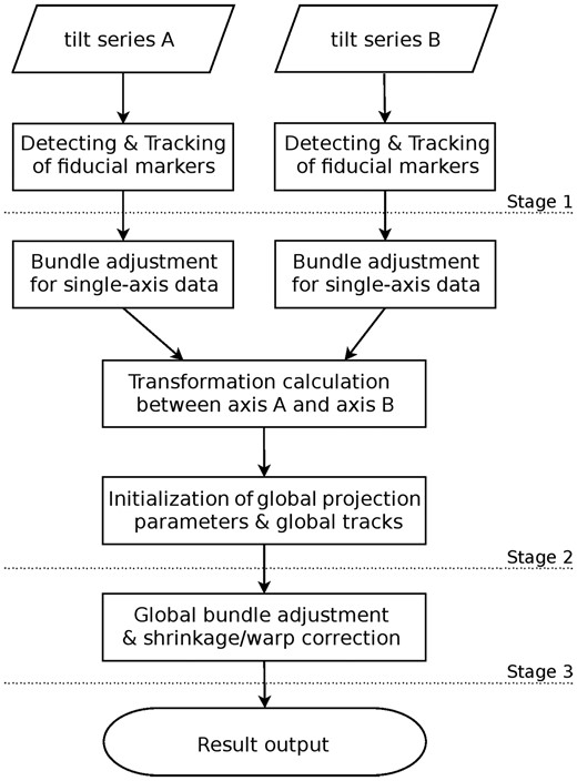
The workflow of fully automatic simultaneous alignment scheme

2.1 Detection and tracking of fiducial markers

2.1.1 Fiducial marker detection

In our proposed workflow, the fiducial marker detection is reduced to a sampling and clustering problem, which is composed of three main steps: (i) fiducial marker diameter estimation, (ii) fiducial marker position detection, and (iii) fiducial marker position refinement. Figure 2 summarizes the entire workflow of fiducial marker detection.

Fig. 2.

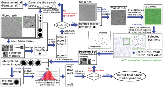
The workflow of fiducial marker detection

Diameter estimation: The accuracy of the fiducial marker diameter is important and has a great influence on the localization precision. Our procedure automatically refines the diameter at the beginning. The fiducial marker diameter estimation relies on the assumption that a good diameter value will output stable diameter detection. Firstly, the $0^{°}$ micrograph is chosen and different values of the marker diameters are guessed and used to detect the fiducial markers. For each diameter value, the similarity of the detected fiducial markers with the artifact fiducial marker template is calculated. Then the guessed diameters are ranked with the overall similarity, and the diameter value with the highest similarity is recorded. Repeating the procedure and narrowing the search space would finally produce the diameter value with the highest similarity as the fiducial marker diameter.

Position detection: Given a known fiducial marker diameter value, the number of clearly localized fiducial markers is upper-bounded for a micrograph (the capacity is fixed by $w·h/d^2$⁠, where w is the width of the micrograph, h is the height of the micrograph and d is the fiducial marker diameter). Here, the fiducial marker detection problem is further reduced to a sampling and clustering problem in our procedure.

Sampling: An average fiducial marker template (denoted as T_avg) from the low-tilt micrograph can be gained in the previous process. With the average template T_avg, a cross-correlation between the fiducial marker template and the micrograph can be calculated. By dividing the correlation matrix of the micrograph into subareas with size d × d and searching the maximum value in each subarea, a number of $(w·h)/d^2$ peaks can be picked. These peak positions are the candidates for fiducial marker positions.

Clustering: Each peak has the correlation value as the score of shape similarity and the pixel value as the score of contrast similarity. The two scores compose a feature space for the candidates, in which the detected positions can be grouped into two clusters, i.e. the fiducial marker cluster and the background (non-fiducial marker) cluster. Here, it should be noticed that there are thousands of background points. Observing from the central limit theorem, the background follows a Gaussian-like distribution in the feature space. Consequently, an expectation-maximization (E-M) clustering with the Gaussian mixture model is carried out to separate the fiducial markers from the background points. For a detected peak, two probabilities are produced indicating how likely the peak belongs to the fiducial marker cluster or the background cluster, respectively. With such clustering, the fiducial markers can be detected fully automatically and exhaustively. More detailed descriptions can be found in Supporting Information Section S1.1.

Position refinement: Considering the scale and defocus difference of each micrograph, the detected fiducial markers are refined with the assumption that the appearance of the fiducial markers in one micrograph is similar to each other. Firstly, an average template of the fiducial markers is generated from the detected fiducial markers that belong to an identical micrograph. Then the peak deviations between each of the fiducial markers and the average template are calculated. For each fiducial marker position, by recalculating the position with the deviation, new fiducial marker positions can be generated, leading to the corresponding new average template. Repeat the above procedure until the total deviation between the fiducial markers and the average template reduces below a threshold (a stable minimal residual). Hereby, the fiducial marker positions are refined consistently with the scale and defocus change of the corresponding micrograph.

2.1.2 Fiducial marker tracking

According to the most recent proof of the relationship between the projection model and the tracking model (Han et al., 2018), the positions of fiducial markers on two micrographs are related by affine transformation within a very small deviation, which makes it possible to track the fiducial markers only based on their two-dimensional (2D) projections. Here, the fiducial marker tracking problem is reduced to an incomplete point set registration problem:

Let ‘point set’ denote the positions of the fiducial markers extracted from a projection. Given two point sets (⁠$\mathcal{M}$ and $\text{S}$⁠) belonging to different views, an affine transformation $\mathcal{T}(·)$ applied to the moving ‘model’ point set $\mathcal{M}$ can be found so that there exists a subset of $\mathcal{T}(\mathcal{M})$ with the maximum cardinality in which the points are corresponding to the points from a subset of the static ‘scene’ set $\text{S}$ under a selected measure of distance.

Two different tracking algorithms are implemented in our proposal: (i) the RANSAC-based tracking algorithm (Han et al., 2015) that can ensure the robustness to noise with relatively slow execution time, and (ii) the fast tracking algorithm (Han et al., 2018) that solves the tracking problem by algebraic optimization. The main ideas of the two algorithms are summarized as follows:

In the RANSAC-based tracking algorithm, the point sets from two different projections are divided into the ‘query set’ and the ‘reference set’. Firstly, a query tree based on the four-point-set (A set of four points on one surface consist a system that keeps the cross-ratio invariant under affine transformation.) (Aiger et al., 2008) for the reference set is built. Here, only the four points with wide-baseline are used. Then a four-point-set is randomly selected from the query set, which is queried in the query tree. If the closest peer is obtained, a transformation can be calculated from the two corresponding four-point-sets. If the estimated transformation is not degenerate and can cover enough points, the transformation is recorded as a candidate of the global transformation between the query set and the reference set. Repeat the procedure until there is no improvement of the transformation’s mapping residual or it reaches the termination of the consensus query.

In the fast tracking algorithm, the point sets are represented by the probability density function of a Gaussian kernel, i.e. the Gaussian-mixed model (GMM). The algebraic solution contains two steps. Firstly, the affine transformation parameters are coarsely refined based on the theoretical transformation derived from the projection model and its 2 D projections (Han et al., 2018). This step can ensure the existence of the solution and give a coarse estimation of the global affine transformation. Then, the transformation parameters are refined based on the GMM-presented point set and coherent point drift technique (Myronenko and Song, 2010). These steps can provide a fitted estimation in an E-M fashion.

In general, the RANSAC-based algorithm is robust but slow, while the algebraic algorithm is fast but slightly less robust. Here, the merits of the two algorithms can compensate each other. Considering the mass of fiducial markers in the view of large field, fast fiducial marker tracking is recommended since it is much faster than the random sampling algorithm. If the fast tracking fails for two attempts with different initializations, the procedure will automatically alter to the RANSAC-based tracking. However, in most cases, the fast tracking is robust enough to go through the entire procedures fluently. More details about the two tracking algorithms can be found in Supporting Information Section S1.2.

2.2 Combination of two tilt series

With the exhaustive detection and tracking of the fiducial markers, it is possible to fully use the information of the mass tracks to recover the projection parameters as well as the optical distortion. Before the global optimization, a combination of the two tilt series is required.

2.2.1 Projection parameters pre-refinement

Each tilt series is aligned separately before the combination. Firstly, it is straightforward to fix the large motion of two different views by using the information of affine transformation. For example, given the already known affine transformation of the two views, i.e. $x\prime =Ax+t$ (A is a 2 × 2 transformation matrix, t is a 2 × 1 translation vector, x is the fiducial marker position from one projection and $x\prime$ is the corresponding marker position from the other projection), the invariant point $x_0$ that makes $x_0=A{x}_0+t$ is the point that can minimize the difference between $\{x\prime \}$ and $\left\{x\right\}$⁠. Furthermore, considering the invariant of tilt axis, the in-plane rotation can also be compensated by analysis of multiple tracks.

Then, the 3 D relationship of the micrographs in one tilt series is considered. As a practical implementation, the projection is modeled as a classic orthogonal projection (The bold font is used to indicate vectors or matrices; a 2D point is represented by a 2 × 1 vector.):

$$\begin{array}{l}\left(\begin{array}{c}u\\ v\end{array}\right)=s{R}_{\text{γ}}P{R}_{\text{β}}{R}_{\text{α}}\left(\begin{array}{c}X\\ Y\\ Z\end{array}\right)+t,\\ R_{\text{α}}=\left(\begin{array}{ccc}1& 0& 0\\ 0& \cos \text{α}& \sin \text{α}\\ 0& -\sin \text{α}& \cos \text{α}\end{array}\right),\\ R_{\text{β}}=\left(\begin{array}{ccc}\cos \text{β}& 0& -\sin \text{β}\\ 0& 1& 0\\ \sin \text{β}& 0& \cos \text{β}\end{array}\right),\\ P=\left(\begin{array}{ccc}1& 0& 0\\ 0& 1& 0\end{array}\right),\\ R_{\text{γ}}=\left(\begin{array}{cc}\cos \text{γ}& \sin \text{γ}\\ -\sin \text{γ}& \cos \text{γ}\end{array}\right),\end{array}$$

(1)

where s is the image scale change, γ is the inplane rotation angle, α is the pitch angle of the tilt axis, β is the tilt angle of the sample, (u, v) is the measured projection point and P denotes the orthogonal projection matrix. The projection parameters can be optimized by the procedure described in Section 2.3.2.

2.2.2 Spatial relationship calibration

The two separately refined tilt series should be merged into a single global coordinate system. Here, the calibrated spatial fiducial markers $\left\{{(X,Y,Z)}^T\right\}$ serve as the bridge of tilt series A and tilt series B.

Denote the spatial fiducial markers calibrated in tilt series A as ${\mathcal{X}}^A=\left\{X_j^A\right\}$ and that in tilt series B as ${\mathcal{X}}^B=\left\{X_j^B\right\}$⁠. Theoretically, the corresponding fiducial markers in ${\mathcal{X}}^A$ and ${\mathcal{X}}^B$ have a relationship of rigid transformation. However, due to the optical distortion and local optimization, ${\mathcal{X}}^A$ and ${\mathcal{X}}^B$ cannot be simply related by rigid transformation. An affine transformation is much more feasible to describe the relationship between ${\mathcal{X}}^A$ and ${\mathcal{X}}^B$⁠. Considering the possibility of view field’s difference, the 3 D point set registration based on RANSAC is used (it is a 3 D version of the algorithm described in Supporting Information Section S1.2.1, by extending the model from 2 D to 3 D).

After obtaining the corresponding relationship, we denote the matched spatial fiducial markers from tilt series A as ${\mathcal{P}}^A={\left\{r_n^A\right\}}_{n=1,\mathrm{...},K}$ and the corresponding ones as ${\mathcal{P}}^B={\left\{r_m^B\right\}}_{m=1,\mathrm{...},K}$⁠, where K is the number of fiducial markers. With the merging pairs $(r_i^A,r_i^B)$⁠, a rigid transformation $\mathcal{T}(·)$ from ${\mathcal{P}}^A$ to ${\mathcal{P}}^B$ that approximates the affine transformation can be calculated by the least square estimation.

For the convenience of discussion, we define the coordinate system of tilt series A as the global coordinate system. Given a rigid transformation that makes $r^B=R_{\text{rigid}}{r}^{A\prime }+t_{\text{rigid}}$⁠, where $R_{\text{rigid}}$ and $t_{\text{rigid}}$ are the approximate estimation of the rigid transformation from $r^A$ to $r^B$⁠, and $r^{A\prime }$ is the inversion estimation of $r^A$ from ${\mathcal{T}}^{-1}(r^B)$⁠, the parameters and spatial fiducial markers to describe the projection of axis B under the coordinate system of A can be denoted as:

$$\left(\begin{array}{c}{u}_B\\ v_B\end{array}\right)=s_B{R}_{{\text{γ}}_B}P{R}_{{\text{β}}_B}{R}_{{\text{α}}_B}\left(R_{\text{rigid}}{r}^{A^{\prime }}+t_{\text{rigid}}\right)+t_B.$$

(2)

By considering the observation of projection ${(u_B,v_B)}^T$ on the coordinate system of A, we have:

$$\left(\begin{array}{c}{u}_B\\ v_B\end{array}\right)=s_{A\prime }{R}_{{\text{γ}}_{A\prime }}P{R}_{{\text{β}}_{A\prime }}{R}_{{\text{α}}_{A\prime }}{r}^{A^{\prime }}+t_{A\prime }.$$

(3)

The initial transformation for each micrograph in tilt series B is estimated separately. By substituting Equation (2) to Equation (3) and solving a non-linear least square problem, we can get the corresponding initial estimation of the global parameters $s_{A\prime },{\text{γ}}_{A\prime },{\text{β}}_{A\prime },{\text{α}}_{A\prime },t_{A\prime }$⁠, with which the projection in tilt series B can be represented under the coordinate system of A for the consequent global optimization (a detailed solution can be found in Supporting Information Section S1.3). Furthermore, with the relationship between the spatial fiducial markers of A and B, it is easy to generate globally consistent tracks that go across both tilt series. The tracks that cover enough micrographs in one tilt series are also kept for the further analysis.

2.3 Global optimization of the tilt series

With the globally transformed projection parameters and tracks, a global optimization of the two tilt series can be solved, based on which a simultaneous reconstruction will be carried out.

2.3.1 Globally consistent model

The separate alignment and reconstruction cannot remove the ambiguity in the parameter optimization for tilt series A and B (Cantele et al., 2010). Here, a two-stage based projection parameter estimation is designed to produce the global optimization.

In the first stage, a simultaneous alignment based on the orthogonal projection model is carried out, as shown in Equation (4):

$$\left(\begin{array}{c}{u}_{\text{G}}\\ v_{\text{G}}\end{array}\right)=s_{\text{G}}{R}_{{\text{γ}}_{\text{G}}}P{R}_{{\text{β}}_{\text{G}}}{R}_{{\text{α}}_{\text{G}}}\left(\begin{array}{c}X\\ Y\\ Z\end{array}\right)+t_{\text{G}}.$$

(4)

Here, to distinguish from the prealignment, the suffix G is used to denote global parameters and to announce that all the parameters of the two tilt series are optimized under a single global coordinate system. Firstly, the spatial fiducial marker estimation is fixed to the value from tilt series A and the parameters from tilt series B are adjusted. After the initialization, the parameters are relaxed to be subject to tuning for both tilt series A and tilt series B. By doing this, the ambiguity caused by the unknown depth in the separate estimation can be removed.

However, due to the optical distortion, the orthogonal projection model is not enough to produce a consistent, global alignment. In the second stage, an extended projection model with extended parameters is introduced to cope with the issue:

$$\left(\begin{array}{c}{u}_{\text{G}}\\ v_{\text{G}}\end{array}\right)=R_{{\text{γ}}_{\text{G}}}P{R}_{{\text{β}}_{\text{G}}}{R}_{{\text{α}}_{\text{G}}}\left(\begin{array}{ccc}{\text{ω}}_x& 0& 0\\ 0& {\text{ω}}_y& 0\\ 0& 0& {\text{ω}}_z\end{array}\right)\left(\begin{array}{c}X\\ Y\\ Z\end{array}\right)+t_{\text{G}},$$

(5)

where ω_x, ω_y and ω_z are the distortion weight along the x, y, z directions, respectively. Here, all the parameters from axis A and axis B are free for optimization. Therefore, the information inherent in both tilt series determines the optimization simultaneously.

2.3.2 Robust estimation

An L-2 norm objective function is used to optimize the parameters:

$$E={\displaystyle \sum _i{\displaystyle \sum _j{\left({\text{Proj}}_i(X_j)-x_{i,j}\right)}^2}}{\text{δ}}_{i,j},$$

(6)

where $\mathcal{X}=\left\{X_j\right\}$ is the set of spatial points to be estimated, $\text{Proj}(·)$ is the process of projection defined in Equations (4) and (5) [also feasible for Equation (1)], and $x_{i,j}$ is the configured position of fiducial marker and ${\text{δ}}_{i,j}$ (⁠${\text{δ}}_{i,j}\in \{0,1\}$⁠) indicates whether the j-th marker is visible in the i-th micrograph. Our aim is to find the most appropriate projection parameters to minimize the objective function E as well as to produce the estimation of spatial fiducial markers.

For the robustness of the estimation, the projection parameters are refined incrementally from the orthogonal projection to the distortion compensated projection. A sparse version of bundle adjustment (SBA) (Triggs et al., 2000) is adapted and a procedure against noise is proposed to solve this problem:

1. Initialize $\mathcal{X}$ by backprojection of $\left\{x_{i,j}\right\}$⁠;

2. Optimize projection parameters in Equation (4) by SBA;

3. For the i-th micrograph, reproject every $X_j$ by the i-th projection parameters and calculate the deviation with measured positions;

4. Calculate the threshold and remove the positions with large deviations (outliers);

5. Repeat Steps 2–4 until no outliers are removed.

If Equation (4) converges, the procedure introduces parameters for distortion correction, moves to Equation (5), and iterates until convergence. Here, a threshold based on M-estimator is used to suppress the effect of noise. And the orthogonal projection uses a relatively relaxed threshold to retain distortion information. More details can be found in Supporting Information Section S1.4.

2.3.3 Simultaneous reconstruction

Projection-model-altered versions of SART and SIRT are provided to solve the simultaneous reconstruction of distortion-extended projection model. Both SIRT and SART are algebraic reconstruction methods. Algebraic reconstruction methods formulate the 3 D reconstruction problem as a large system of linear equations, which guarantees the ability to model the inverse projection problem discretizing the geometric optics models of the image formation process.

In the following, we adopt a discrete representation of the space: volume reconstructions are made of voxels, with u_j representing the unknown density value and N the total number of voxels. The projection constraints are then expressed with the following linear system:

$$v_i={\displaystyle \sum _i^M{w}_{i,j}}{u}_j,$$

(7)

where v_i denotes the i-th measured projection value and $M=B\times S$ is the dimension of v, B being the number of projection angles and S the number of projection values per view. The matrix $W={(w_{i,j})}_{M\times N}$ is a sparse matrix where $w_{i,j}$ can be computed according to the contribution of the j-th point in the volume to the i-th projection, once the projection map is specified.

Before reconstructing the volume $u_j$⁠, we should first define the matrix W. In our projection-model-altered version, the matrix W is defined by the $\text{Proj}(·)$ discussed above, i.e. extended projection model with parameters for distortion correction. For SART (Andersen and Kak, 1984; Castaño-Díez et al., 2007), the iterative process with extended projection model can be written by the following expression:

$$u_j^{(k+1)}=u_j^k+{\displaystyle \sum _{i=1}^S\frac{\text{λ}{w}_{i,j}}{{\displaystyle {\sum }_{i=1}^S{w}_{i,j}}{\displaystyle {\sum }_{h=1}^N{w}_{i,h}}}\left(v_i(P_b(j))-{\displaystyle \sum _{h=1}^N{w}_{i,h}}{u}_h^k\right)},$$

(8)

where k is the index of the iteration, λ is the relaxation factor (in general, $0<\text{λ}<2$⁠), $i=bS+s$ denotes the i-th equation of Equation (7) and $b=(k\mathrm{mod}B)$ is the index of the view. SART adopts a view-by-view strategy. That is, an approximation is updated simultaneously by all the projections of each view. SIRT (Gilbert, 1972; Sorzano et al., 2001) is another type of iterative reconstruction method, which uses all the projections from all the views in each iteration.

3 Experiments and results

3.1 Datasets

Two experimental datasets are used here to show the performance and improvement by simultaneous alignment. In the following context, we will call the tilt series generated from the relatively vertical tilt axis as ‘axis A’ and the ones generated from the relatively horizontal tilt axis as ‘axis B’.

The first dataset, Centriole, is a tilt series of plastic embedded cell section around a centriole region, which was taken on a FEI TF30 microscope (operated at 300 kV) with a Gatan Camera. The 0-degree tilt image of the tilt-series A and B are illustrated in Figure 3(A) and (D), respectively. This dataset is obtained from IMOD tutorial (Downloaded from http://bio3d.colorado.edu/imod/files/tutorialData-1 K.tar.gz). The tilt angles of the projection images range from $+{65.0}^{°}$ to $-{61.0}^{°}$ at $2^{°}$ intervals. There are 64 images in the tilt series of each axis. The size of each tilt image is 1024 × 1024 with a pixel size of 1.01 nm. The initial orientation of the tilt azimuth with respect to the vertical direction of the images from axis A and axis B is $-{12.5}^{°}$⁠.

Fig. 3.

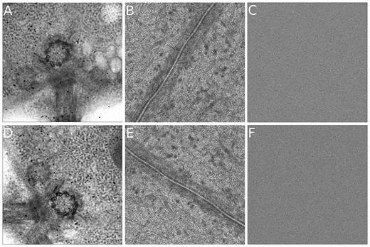
Illustration of test datasets. (A)&(D) The $0^{°}$ micrographs of Centriole of axis A and axis B. (B)&(E) The $0^{°}$ micrographs of Adhesion belt of axis A and axis B. (C)&(F) The $0^{°}$ micrographs of simulated dataset of axis A and axis B

The second dataset, Adhesion belt, is a tilt series of the adhesion belt structure. The Adhesion belt dataset was a negative stained cryo-ET dataset provided by the National Institute of Biological Sciences of China. The data were collected by an FEI Titan Krios (operated at 300 kV) with a Gatan camera. The 0-degree tilt images of the tilt-series A and B are illustrated in Figure 3(B) and (E), respectively. There are 111 images for axis A and 113 images for axis B, with tilt angles ranging from $-{60.0}^{°}$ to $+{60.0}^{°}$ at 1–2° intervals for each axis. The size of each tilt image is 2048 × 2048, with a pixel size of 2.03 nm (two magnitude-binned). The initial orientation of the tilt azimuth with respect to the vertical direction of the images from axis A and axis B is ${2.4}^{°}$⁠. This dataset has a mass of fiducial markers embedded in the specimen.

Due to the lack of resolution criteria in ET (Cardone et al., 2005), it is difficult to directly measure the resolution improvement by experimental data. Here, a simulated dataset (named as Simul) generated by InSilicoTEM (Vulović et al., 2013) is used to demonstrate the reconstruction improvement of our toolkit. The simulated tomogram with $2560\times 2560\times 250$ voxel that contains 81 volumes of 2WRJ (the default map in InSilicoTEM, downsampled by two factor) was generated. And about 45 fiducial markers with a diameter of 18 pixels were embedded. From the tomogram, 51 projections were produced for each tilt axis (⁠$+{50.0}^{°}$ to $-{50.0}^{°}$ at $2^{°}$ intervals), and random translation and rotation ranging in ±150 pixels and $\pm {10}^{°}$ were added. The 0-degree tilt images of the tilt-series A and B are illustrated in Figure 3(C) and (F), respectively. More details of the simulation process can be found in Section S2.1. This simulated dataset is processed by subtomogram averaging to further demonstrate the effect of simultaneous reconstruction in resolution. Because the 2WRJ map has been downsampled by two factor in our simulation, in the following analysis, we assume that both the micrograph and the ground-truth are obtained with 2 Å per pixel.

Table 1 summarizes the parameters of all the datasets.

Table 1.

Parameter summary of the datasets

Dataset	Centriole	Adhesion belt	Simulation
Microscope	FEI TF30 (300 kV)	Titan Krios (300 kV)	Ideal (300 kV)
Tilt range	$+{65}^{°}\text{to}-{61}^{°}$	$-{60}^{°}\text{to}+{60}^{°}$	$+{50}^{°}\text{to}-{50}^{°}$
Interval	$2^{°}$	1 to $2^{°}$	$2^{°}$
Image size	1024 × 1024	2048 × 2048	2560 × 2560
Pixel size	10.1 Å/pixel	20.3 Å/pixel	2.0 Å/pixel

Both SART and SIRT implementation based on C++/MPI with the distortion-extended projection model are provided in our toolkit. However, without loss of generality, in the following context, only the results based on SART are shown.

3.2 Results

3.2.1 Automatic detection and tracking

Fiducial marker detection and tracking are the basis of marker-based alignment. Here we use the Centriole dataset to demonstrate the automatic detection and tracking in our workflow.

Figure 4 shows the detected fiducial markers from the projection images at $0^{°}$ and a high tilt angle. As shown in Figure 4(A) and (C), all the well-distributed markers at low tilt angles are detected by our workflow. In addition, most of the good-shape fiducial markers in high tilt angles are detected [Fig. 4(B) and (D)], whereas the blurred and low-contrast fiducial markers are excluded, which indicates the robustness of our marker detection procedure. For the entire tilt series in the two axes, our method detects more than 90% of the fiducial markers.

Fig. 4.

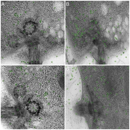
Illustration of marker detection. All the detected markers are marked by circles. (A) Detected fiducial markers from the micrograph of axis A with $0^{°}$ tilt angle. (B) Detected fiducial markers from the micrograph of axis A with ${64}^{°}$ tilt angle. (C) Detected fiducial markers from the micrograph of axis B with $0^{°}$ tilt angle. (D) Detected fiducial markers from the micrograph of axis B with ${64}^{°}$ tilt angle

The length of the tracks is used to demonstrate the overall performance of the detection and merging. Figure 5 demonstrates the histograms of the tracking length obtained by the tracking procedure. In our implementation, the projection images with one or two view intervals are matched and then combined into several merging pairs to obtain the tracks. Not all the markers will go across the entire tilt series and the micrographs at high tilt angles will have more fiducial markers, as shown in Figure 5 (A) and (B). For the tilt-series of axis A, we detected 25 tracks that cover the entire tilt series. For the tilt-series of axis B, we detected 28 tracks appearing in the entire tilt series. We obtained 21 tracks (fiducial markers) whose projections appear both in the tilt series of axis A and axis B [Fig. 5(C)]. There are 14 tracks that cover the entire tilt series of both axis and the length of all the 21 tracks is higher than 100 (128 micrographs in total). By analyzing the overlapped space of the tilt series of axis A and axis B, we can find that all the fiducial markers that appear both in the tilt series of axis A and axis B are identified and tracked.

Fig. 5.

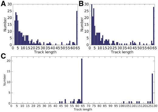
(A) The track lengths of tilt series of axis A. (B) The track lengths of tilt series of axis B. (C) The combined track lengths of tilt series of axis A and B

3.2.2 Tilt series combination

With the mass of fiducial marker tracks, it is possible for us to fix the optical distortion. In our strategy, we used all the well tracked fiducial markers (the tracks that cover more than 85% of the micrographs for each tilt series) in both axis A and axis B. Figure 6 demonstrates the tracks for datasets Centriole and Adhesion belt, after the pre-refinement of projection parameters. As showed in Figure 6(A) and (B), the shift and rotations are almost corrected, and both the tile series A and B are aligned under a single unique coordinate system. Our model does not assume the relative locations of the two tilt axes. Instead, it treats the tilt based on the value of Euler angles that are recalculated from the information of the tilt angles. The relationship of each tilt series can be discovered automatically in our scheme.

Fig. 6.

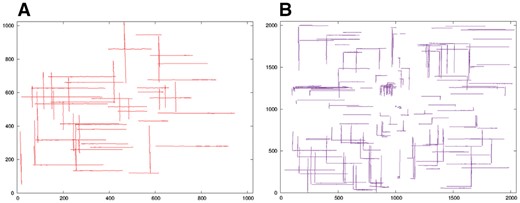
Illustration of pre-refinement of projection parameters. (A) Overlay of the pre-refined fiducial marker tracks of dataset Centriole. (B) Overlay of the pre-refined fiducial marker tracks of dataset Adhesion belt

3.2.3 Global optimization and reconstruction

If the axis A and B are calibrated under a single global coordinate system but just based on the orthogonal projection model, the inconsistency caused by optical distortion still remains. We illustrate the difference between the global optimization based on the orthogonal projection model and the projection model with distortion correction in Figure 7. Without distortion correction, the reconstructed fiducial markers have ambiguous shapes [Fig. 7(A)], whereas distortion correction results in well-shaped markers and fewer artifacts [Fig. 7(B)].

Figure 8 demonstrates the final reconstruction of Centriole by both AuTom-dualx and IMOD (Because it is difficult and unfair to compare the results from different reconstruction methods (for example, WBP and SART), the weighted back-projection (WBP) in the workflow of IMOD is replaced by SART, with all the geometry parameters unchanged.). Here, AuTom-dualx uses the simultaneous alignment and reconstruction procedure, and IMOD separately reconstructs the two axes and then merges the reconstruction together. It can be seen that the result of AuTom-dualx is smoother than that of IMOD, and there are less artifacts in the result of AuTom-dualx on the top slice. The average reprojection residual of fiducial markers for the global estimation in AuTom is 0.516, whereas the average fiducial marker reprojection residuals of tilt series A and B for IMOD are 0.556, 0.591, respectively (The reprojection residual can only prove the alignment quality to a certain extent, because the projection models used in AuTom and IMOD are different.). We further compared the reconstruction by reprojection consistent analysis. We find that the average normalized cross-correlation (NCC) value of AuTom-dualx’s reprojection with the original two tilt series (the center 512 × 512 area) is 0.955 while that of IMOD for axis A and axis B is 0.953 and 0.951, respectively (IMOD can only ensure the consistency in one axis).

Fig. 7.

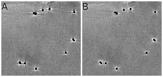
Reconstruction results of the lefttop part of Centriole (SART with 40 iterations and relaxation factor $\text{λ}=0.2$⁠). (A) Reconstruction of the alignment based on the classic orthogonal projection. (B) Reconstruction of the alignment with distortion correction

Fig. 8.

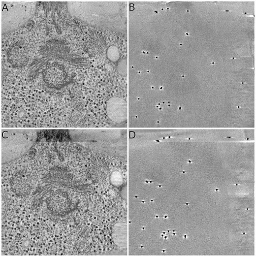
Sample slices of reconstruction on the Centriole dataset. All the illustrated data are reconstructed by SART with 40 iterations and relaxation factor $\text{λ}=0.2$⁠. (A)&(B) The middle and top slices of the reconstruction obtained by the simultaneous alignment and reconstruction of AuTom-dualx. (C)&(D) The middle and top slices of the reconstruction obtained by the separate reconstruction and merging of IMOD (merging axis B to axis A)

Figure 9 shows the final reconstruction of Adhesion belt by both AuTom-dualx and IMOD. The result of AuTom-dualx has a higher contrast and clearer details. The average reprojection residual of fiducial markers for the global estimation in AuTom is 0.69, whereas those of tilt series A and B for IMOD are 0.915 and 0.945, respectively. By reprojection consistent analysis, we find that the average NCC value of AuTom-dualx’s reprojection with the original two tilt series (the center 1024 × 1024 area) is 0.916 while that of IMOD for axis A and axis B are 0.906 and 0.911, respectively.

For these two datasets, a detailed comparison of selected fiducial markers are shown in Figure 10, in which the top panel is the results produced by AuTom-dualx and the bottom one is produced by IMOD. From the shape of the fiducial markers, we can find that the results produced by simultaneous alignment and reconstruction show fewer artifacts and less elongation, especially along the direction of missing wedge.

Fig. 9.

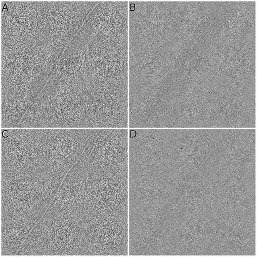
Sample slices of reconstruction on the Adhesion belt dataset. All the illustrated data are reconstructed by SART with 40 iteration and relaxation factor $\text{λ}=0.2$⁠. (A)&(B) The middle and top slices of the reconstruction obtained by the simultaneous alignment and reconstruction of AuTom-dualx. (C)&(D) are the middle and top slices of the reconstruction obtained by the separate reconstruction and merging of IMOD (merging axis B to axis A)

Fig. 10.

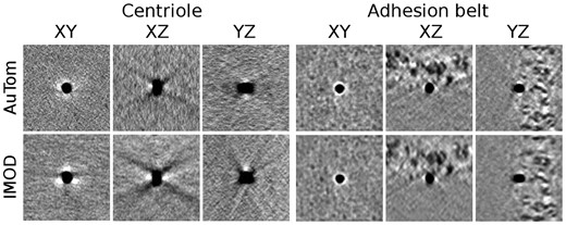
Fiducial marker subvolumes from the Centriole (left) and Adhesion belt (right) datasets. The fiducial marker location in the Centriole volumes is (449 418 259) for AuTom-dualx and (475 418 283) for IMOD. The fiducial marker location in the Adhesion belt volumes is (578 1025 116) for AuTom-dualx and (574 1035 105) for IMOD

We further studied the reprojection consistency (Fig. 11). Here, because IMOD uses a separate reconstruction and merging strategy, there are two choices, i.e. merging the reconstruction of axis B to the one of axis A or merging the reconstruction of axis A to the one of axis B. IMOD can only keep the consistency for one tilt series, whereas AuTom-dualx calibrates the projection parameters and reconstruction of axis A and axis B simultaneously. Therefore, AuTom-dualx can well balance the consistency between axis A and axis B. For IMOD on the Centriole dataset, when merging axis B to axis A, the average NCC value for the micrographs in axis A can reach 0.953 while that in axis B is only 0.878. On the contrary, when merging axis A to axis B, the average NCC value for the micrographs in axis B can reach 0.951 while that in axis B is only 0.863. As a comparison, the results of AuTom-dualx always keep high NCC values and gain an average value of 0.955. A similar conclusion can be drawn for the Adhesion belt dataset [Fig. 11(B)]. For IMOD, when merging axis B to axis A, the average NCC value for the micrographs in axis A can reach 0.906 while that in axis B only reaches 0.809; when merging axis A to axis B, the average NCC value for the micrographs in axis B can reach 0.911 while that in axis B only reaches 0.812. AuTom-dualx can keep a consistent NCC value of 0.916. It is interesting that AuTom-dualx obtains a better correlation value on axis B and IMOD has a large decline when merging B to A. This is due to the tilt range difference: axis B has 113 micrographs and series A has 111 micrographs, axis B thus has more contribution to the 3 D reconstruction and better NCC values.

Fig. 11.

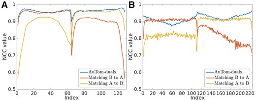
The NCC curves between the reprojection of the reconstruction for both AuTom-dualx and IMOD and the original tilt series for the Centriole dataset (A) and the Adhesion belt dataset (B)

3.2.4 Resolution gain by simultaneous reconstruction

Reprojection consistency represents one aspect of the reconstruction results. A more direct measurement is the reconstruction resolution. However, unlike Fourier shell correlation (FSC) in single particle cryo-EM, the field of ET still lacks such mature criteria (Cardone et al., 2005). Here, the experiment of a simulated tomogram that contains several copies of the already-solved ribosome structure (2WRJ) was designed to evaluate the reconstruction resolution.

Firstly, the dataset Simul was aligned and reconstructed by the workflow of IMOD and AuTom-dualx respectively, with SART (20 iterations, $\text{λ}=0.2$⁠). For each workflow, a reconstructed tomogram that contains all the 81 substructures was obtained. Then the subvolumes that contain the ultrastructure were selected. Since the rotation and translation for each subvolume are known in Simul, it is not difficult to obtain an accurate averaged subtomogram from the picked subvolumes by inverse transformation (Considering the radiation damage caused by the electron beam, it is not natural to use dual-axis tomogram in subtomogram averaging. However, the conclusion that is drawn from the simulation is universal from the computational point of view.). For the simulated dataset, since the ground truth is at hand, we compared the optimized fiducial marker positions of AuTom-dualx and IMOD with the ground-truth (Supporting Information Section S2.2).

To analyze the results, both FSC and Resmap (Kucukelbir et al., 2014) were used to compare the performance between AuTom-dualx and IMOD. For each subtomogram, a sphere mask with a diameter of 180 pixels was applied to remove the surrendering area, and the ground-truth of the ribosome (the 2WRJ map) was used as the reference. All the results were calculated with the Å/voxel setting to 2. Figure 12 shows the FSC curves between the reconstructed subtomogram and the reference 2WRJ map of AuTom-dualx and IMOD. According to the frequency value truncated at 0.5 (⁠$FS{C}_{0.5}$⁠), the result of AuTom-dualx has a resolution of 5.49 Åwhile the result of IMOD has a resolution of 5.88 Å. The results obtained by Resmap also draw a similar conclusion. As shown in Figure 13, we can find that most of the local resolutions gained by AuTom-dualx are distributed around 5.4 Å, while the majority of the local resolutions gained by IMOD are distributed around 6.2 Å (This experiment is based on simulation, in which many variables were simplified. The value of resolution presented here is just for the purpose of computational method comparison but not to indicate the advance in subtomogram averaging.). Here, both the results of FSC and Resmap indicate that simultaneous reconstruction can gain an improvement of the reconstruction quality compared to the reconstruction-combination strategy. And the results here are also consistent with the conclusion in Winkler and Taylor (2013).

Fig. 12.

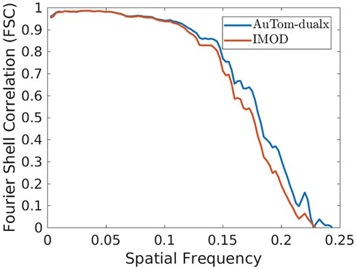
The Fourier shell correlation between the reconstructed subtomogram and the reference 2WRJ map

Fig. 13.

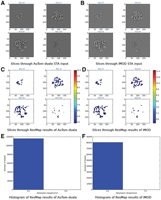
Results obtained by Resmap analysis. (A)&(C)&(E) The slices, local resolution distribution and resolution histogram of the subtomogram produced by the workflow of AuTom-dualx, respectively. (B)&(D)&(F) The slices, local resolution distribution and resolution histogram of the subtomogram produced by the workflow of IMOD, respectively

4 Conclusion

In this paper, we present a toolkit for fully automatic alignment of dual-axis tilt series and simultaneous reconstruction. Our scheme provides the automatic detection and tracking of fiducial markers across the tilt series under large-field datasets, automatic combination of two different tilt series, and simultaneous alignment with inconsistency correction by parameters for distortion correction. The presented toolkit is fully automatic, which does not require manual intervention and avoids the ambiguity in separate alignment. To our knowledge, the presented toolkit is the first general framework for fully automatic alignment of the dual-axis electron tomography, which also produces globally consistent alignment and supports simultaneous reconstruction. The experimental results demonstrate the effectiveness of our workflow.

In the future, we plan to improve the proposed toolkit along the following directions. First, the current toolkit still lacks visualization and auxiliary tools. We will integrate AuTom-dualx into the AuTom platform (Han et al., 2017). The reconstruction acceleration techniques used in AuTom (Wan et al., 2011, 2012, 2013; Zhang et al., 2015) will be migrated to AuTom-dualx to improve the computational efficiency.

Second, we will investigate the effect of the reconstruction strategy under complex conditions, to further accelerate the convergence and improve the reconstruction quality (Tong et al., 2006).

Third, our current toolkit uses extended parameters to correct the optical distortion. Although we have shown that this idea can effectively fix the inconsistency issue in the dual-axis tilt series alignment, a more complex model that considers higher level distortion (Lawrence et al., 2006) is also provided by our toolkit (−w 2 option of dualxmauto), which will introduce $xy,x^2,y^2,xz,yz$ and z² to the distortion correction (Supporting Information Section S1.5). In particular, the work of Myasnikov et al. (2013) supports the wide applicability of dual-axis tomography and the work of Fernandez et al. (2018) further proves the power of distortion correction in single-axis cryo-ET. However, because of the requirement of abundant and well-distributed fiducial markers, the application of higher level distortion correction remains a sophisticated operation in specimen preparation and micrograph-photographing. The high-variance introduced by a complex projection model is also a serious issue, which increases the overfitting risk when the number of fiducial markers is insufficient and the quality of fiducial markers is not so good. Therefore, our toolkit uses a simpler model as default to handle optical distortion, following the Occam’s razor principle. We will further conduct a more comprehensive comparison about the different models under different situations.

Fourth, a potential topic is the application of dual-axis tomography to practical subtomogram averaging. The subtomogram averaging applications, including datasets like EMPIAR-10064 (Khoshouei et al., 2017) and EMPIAR-10045 (Bharat and Scheres, 2016), are becoming more and more popular in structural biology. However, these datasets are all based on single-axis tomography. Currently, there are almost no such applications and datasets that produce subtomogram averaging data based on dual-axis tomography. Theoretically, dual-axis tomography can retain more information for a single particle. Therefore, it is possible for dual-axis based subtomogram averaging, with the development of the instrument, to reduce the radio damage caused by the long time exposure. We will investigate the effect of simultaneous alignment and reconstruction in practical subtomogram averaging if such datasets become available in the future.

Acknowledgements

The authors thank Wanzhong He from National Institute of Biological Sciences, Beijing, China for providing the Adhesion belt dataset.

Funding

This work was supported by the National Key Research and Development Program of China (2017YFE0103900, 2017YFA0504702), the King Abdullah University of Science and Technology (KAUST) Office of Sponsored Research (OSR) under Awards No. FCC/1/1976-04, URF/1/2601-01, URF/1/3007-01, URF/1/3412-01 and URF/1/3450-01. the National natural Science Foundation of China (Grant No. U1611263, U1611261, 61472397, 61502455, 61672493), and Special Program for Applied Research on Super Computation of the NSFC-Guangdong Joint Fund (the second phase).

Conflict of Interest: none declared.