Multiresolution correction of GC bias and application to identification of copy number alterations

Abstract

Motivation

Whole-genome sequencing (WGS) data are affected by various sequencing biases such as GC bias and mappability bias. These biases degrade performance on detection of genetic variations such as copy number alterations. The existing methods use a relation between the GC proportion and depth of coverage (DOC) of markers by means of regression models. Nonetheless, severity of the GC bias varies from sample to sample. We developed a new method for correction of GC bias on the basis of multiresolution analysis. We used a translation-invariant wavelet transform to decompose biased raw signals into high- and low-frequency coefficients. Then, we modeled the relation between GC proportion and DOC of the genomic regions and constructed new control DOC signals that reflect the GC bias. The control DOC signals are used for normalizing genomic sequences by correcting the GC bias.

Results

When we applied our method to simulated sequencing data with various degrees of GC bias, our method showed more robust performance on correcting the GC bias than the other methods did. We also applied our method to real-world cancer sequencing datasets and successfully identified cancer-related focal alterations even when cancer genomes were not normalized to normal control samples. In conclusion, our method can be employed for WGS data with different degrees of GC bias.

Availability and implementation

The code is available at http://gcancer.org/wabico.

Supplementary information

Supplementary data are available at Bioinformatics online.

1 Introduction

The whole-genome sequencing (WGS) technology is widely used for identifying innate or acquired genetic variations. Nevertheless, the quality of WGS data can be affected by various sequencing biases such as GC bias and mappability bias. These biases affect performance on detection of genetic variations such as copy number (CN) alterations. In case of a cancer study, paired normal control sequencing data can serve for correcting these biases (Teo et al., 2012). Nonetheless, both tumor and normal control sequencing data should be generated under the same conditions. Another popular method is to adjust the observed depth of coverage (DOC) of a specific genomic window on the basis of the GC proportion of the window (Magi et al., 2012), as shown in the following formula:

$$\mathit{DO}{C}_{i,\mathit{corrected}}=\mathit{DO}{C}_{i,\mathit{raw}}·\frac{\mathit{DO}{C}_{\mathit{average}}}{\mathit{DO}{C}_{i,\mathit{GC}}},$$

(1)

where $\mathit{DO}{C}_{i,\mathit{raw}}$ is the DOC of specific window i, DOC_average is the average DOC of all genomic windows and $\mathit{DO}{C}_{i,\mathit{GC}}$ is the value of DOC reflecting the level of GC bias of window i. The simplest estimation for $\mathit{DO}{C}_{i,\mathit{GC}}$ is to calculate the average DOC of the genomic windows with the same GC proportion as that of window i. The relation between GC proportion and DOCs $\mathit{DO}{C}_{i,\mathit{GC}}$ can be modeled by means of regression models such as LOESS regression (Scheinin et al., 2014) or polynomial regression (Boeva et al., 2011). Some studies (Benjamini and Speed, 2012; Xi et al., 2016) model the GC bias via the number of reads mapped to the genomic position at a nucleotide level rather than the genomic window level. On the other hand, there are no widely accepted methods for modeling GC bias in the DOC signal because the severity of GC bias varies sample to sample, and factors that cause GC bias are not yet fully identified.

In this study, we developed a new GC bias correction method based on multiresolution bias correction named Wabico (WAvelet transform-based BIas COrrection). We used a translation-invariant (TI) wavelet transform (Coifman and Donoho, 1995) to decompose GC-biased original DOC signals. Then, we modeled the relation between GC proportions and DOC of the genomic regions and constructed artificial control DOC, DOC_GC, which reflects GC bias. When we investigated the performance of our proposed method on GC bias correction in simulated sequencing data and real cancer WGS data, Wabico showed better performance in samples with severe bias than the other methods did.

2 Materials and methods

Figure 1 shows the procedure of the Wabico method. For a WGS Binary Alignment Map (BAM) file, the mapped reads within genomic windows are counted. These windows consist of the same number of uniquely mappable positions (Fig. 1a). We decompose the DOC signal of the genomic windows using the TI wavelet transform (Fig. 1b). It produces scaling coefficients and wavelet coefficients. The scaling coefficients represent the average of DOC values between two neighboring regions, and the relation between scaling coefficients and their GC proportion is modeled by LOESS regression (Fig. 1c). The wavelet coefficients denote the difference in DOC values between two neighboring genomic regions, and the relation between the wavelet coefficients and their GC proportions is modeled by two-dimensional (2D) kernel smoothing (Fig. 1d). After fitted coefficients are obtained, DOC_GC values are generated that represent the GC bias embedded in input WGS data (Fig. 1e). These DOC_GC values are used for correcting GC bias at each decomposition level. By checking the criterion based on the amount of direction of changes consistent with the initial direction of GC changes, we determine whether the decomposition stops or not (Fig. 1f). If further decomposition is necessary to take into account broader genomic regions of the DOC values, the current scaling coefficients will be decomposed into a higher level of scaling coefficients and wavelet coefficients. The steps from (b) to (f) are repeated until the stopping criterion is satisfied. Each step will be explained in more detail. Finally, DOC_GC values generated at the highest level that meet the stopping criteria are suggested to correct the GC bias of the raw DOC values.

Fig. 1.

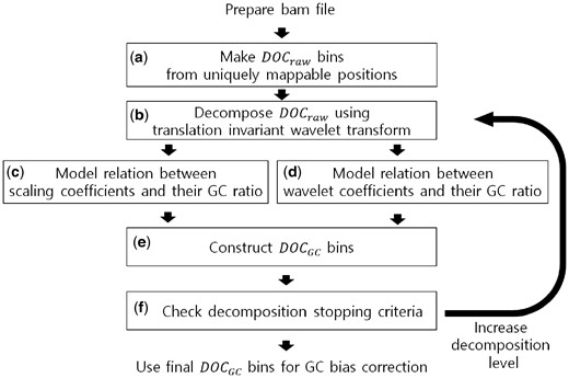
An overview of GC bias correction steps

2.1 CN quantification

The input of Wabico is DOC values obtained from WGS data. DOC is the number of mapped sequencing reads within a given genomic region. In early studies, the size of the genomic region for measuring DOC was fixed (Teo et al., 2012). After that, BIC-Seq2 (Xi et al., 2016) started to use variable-size genomic windows by taking into account the mappability of the sequencing reads. As in BIC-Seq2, we employed variable-size windows containing equal numbers of uniquely mappable positions.

2.2 Decomposition of DOC values via the TI wavelet transform

Raw DOC values are decomposed into wavelet and scaling coefficients using the TI wavelet transform (Coifman and Donoho, 1995) with the Harr wavelet. We chose the TI wavelet transform because it shows better signal recovery performance as compared to the usual discrete wavelet transform (Coifman and Donoho, 1995). At every decomposition level, it utilizes both the given signal and the circularly shifted signal to the right. Figure 2(a–c) shows an example of DOC signal decomposition up to level 2, where the input DOC signal consists of 32 windows. Figure 2(a–c) illustrates the changes of a TI-Table, which is a data structure used in the TI wavelet transform. Given a raw DOC signal [(1) in Fig. 2], it is decomposed into scaling coefficients and wavelet coefficients [(2) and (3) in Fig. 2]. The size of the two resulting coefficients is 16, i.e. a half of the input signal. For maintaining the translation invariance property, a shifted version of the input DOC signal is also decomposed into scaling coefficients and wavelet coefficients [(4) and (5) in Fig. 2]. The scaling coefficients of current level 1 [(2) and (4) in Fig. 2] can be decomposed further into a higher level of scaling coefficients and wavelet coefficients. Figure 2(c) shows the results of decomposition from the TI-Table presented in Figure 2(b). Scaling coefficients (6) and wavelet coefficients (7) come from scaling coefficient (2). Scaling coefficients (8) and wavelet coefficients (9) come from the shifted version of scaling coefficient (2). The sizes of coefficients (6), (7), (8) and (9) are all 8 and a half of the size of coefficient (2) at the previous level 1. Similarly, coefficients (10), (11), (12) and (13) of level 2 come from scaling coefficient (4). In summary, the scaling coefficients of the current level can be decomposed into scaling coefficients and wavelet coefficients of the next level. The detailed procedure is described in the article about the TI wavelet transform (Coifman and Donoho, 1995).

Fig. 2.

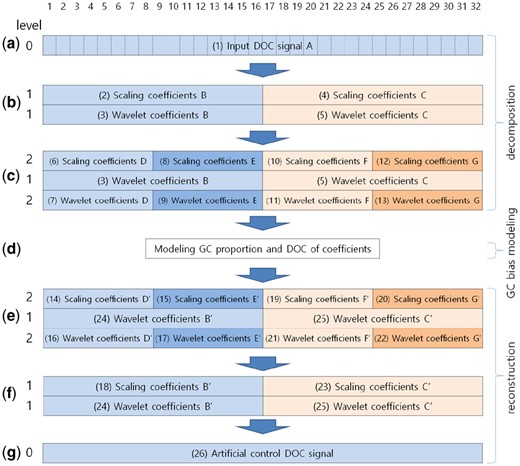
An example of TI-Tables during raw DOC signal decomposition and construction of an artificial control DOC signal. (a) A TI-Table of the input DOC signal consisting of 32 windows. It is a 1 × 32 numerical matrix. (b) The TI-Table after signal decomposition from the input DOC signal (a). This is a 2 × 32 matrix. (c) The TI-Table after signal decomposition of scaling coefficients from (b). TI-Table size is 3 × 32. (d) The modeling step for these coefficients. (e) The TI-Table consisting of fitted coefficients from the previous modeling step. (f) The TI-Table after averaging out of the scaling coefficient and the wavelet coefficient of level 2 in TI-Table (e). (g) The TI-Table containing an artificial control DOC signal after averaging out of the coefficients of TI-Table (f)

2.3 Modeling the relation between scaling coefficients and their GC proportion

After scaling and wavelet coefficients for all given chromosomes are calculated, the relations between these coefficients and their GC proportion are modeled. First, GC proportions for these coefficients are calculated. The scaling coefficient of level 1 covers twice the genomic areas covered by the input signal of level 0. In addition, the scaling coefficient of level j covers twice the genomic areas covered by the scaling coefficient of level j − 1. Every scaling coefficient has its own corresponding GC proportion. The GC proportion of the scaling coefficient for level j is $G{C}_{j,i}=G{C}_{j-1,2i-1}+G{C}_{j-1,2i}$⁠, where i is the index of the coefficient of level j. The GC proportion for the shifted scaling coefficient is $G{C}_{j,i}=\mathit{GC}{\prime }_{j-1,2i-1}+\mathit{GC}{\prime }_{j-1,2i}$⁠, where $\mathit{GC}{\prime }_{j-1}$ is the shifted version of $G{C}_{j-1}$⁠. Supplementary Figure S1 shows an example of GC proportion calculation.

Given all pairs of GC proportion and a scaling coefficient from given chromosomes for level j, LOESS regression (Cleveland, 1979) is used for fitting relation $\mathit{coe}{f}_{\mathit{scaling},j}=\mathit{loess}(G{C}_j)$⁠. The fitted $\mathit{coe}{f}_{\mathit{scaling},j}$ is employed for constructing DOC_GC. The R package limma (Ritchie et al., 2015) provides fast LOESS regression. Figure 3(a) depicts a distribution of raw scaling coefficients and their GC proportions at decomposition level 6 of the simulated data generated by Pysim-sv (Xia et al., 2017) with GC biases at z = 30. The details of the simulated sequence generation will be explained in Section 3. The red curve represents the LOESS-fitted scaling coefficients.

Fig. 3.

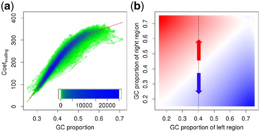
The relation between coefficients and their GC proportions for the simulated GC-biased sequencing reads. (a) The relation between GC proportion and a scaling coefficient. The heatmap represents the distribution of raw scaling coefficients. The x-axis means the GC proportion of the coefficients, and the y-axis denotes the value of the coefficients. Most of scaling coefficients are concentrated in blue areas. The scaling coefficients are rarely distributed in the green areas. The red curve is the LOESS-fitted scaling coefficient depending on the specific GC proportion. (b) The relation between two neighboring GC proportions and a wavelet coefficient. The heatmap indicates the relation between the value of wavelet coefficients (pixel color) and the GC proportion of two neighboring genomic regions (x-axis and y-axis) from 2D kernel smoothing. Red areas represent the increasing DOC values of the right-hand genomic region compared to the left-hand region in the two adjacent genomic regions. The blue areas mean the opposite case

2.4 Modeling the relation between wavelet coefficients and their GC proportion

Wavelet coefficients denote the DOC differences between two neighboring genomic regions in the reference sequence. Because of the difference in GC proportions between the two neighboring genomic regions, a DOC difference between the genomic regions may occur. To construct DOC_GC, the DOC difference should be modeled by means of the GC proportion of the two adjacent regions. The GC proportions of the wavelet coefficients for level j are $G{C}_{\mathit{left},j,i}=G{C}_{j-1,2i-1}$ and $G{C}_{\mathit{right},j,i}=G{C}_{j-1,2i}$⁠, where i is the index of the coefficient of level j. The GC proportions of the wavelet coefficients for the shifted scaling coefficient of previous level j−1 are $G{C}_{\mathit{left},j,i}=\mathit{GC}{\prime }_{j-1,2i-1}$ and $G{C}_{\mathit{right},j,i}=\mathit{GC}{\prime }_{j-1,2i}$⁠, where $\mathit{GC}{\prime }_{j-1}$ is the shifted version of $G{C}_{j-1}$⁠. Supplementary Figure S1 shows an example of GC proportion calculation.

For all the given wavelet coefficients at level j, the relation $\mathit{coe}{f}_{\mathit{wavelet},j}=\mathit{smoother}(G{C}_{\mathit{right},j},G{C}_{\mathit{left},j})$ is modeled, where $\mathit{coe}{f}_{\mathit{wavelet},j}$ is a wavelet coefficient for two adjacent GC proportions $G{C}_{\mathit{right},j}$ and $G{C}_{\mathit{left},j}$ at level j. We used an approximate Nadaraya Watson kernel smoother provided by the smooth.2d function of the R field package (Douglas et al., 2015).

Figure 3(b) shows the smoothed results representing the relation between GC proportions of consecutive genomic regions and wavelet coefficients at decomposition level 6 of the simulated data generated by Pysim-sv (Xia et al., 2017) with GC biases at z = 30. The x-axis represents the GC proportion of the left-hand genomic region, the y-axis represents the GC proportion of the right-hand genomic region and the color represents the value of wavelet coefficients. In this figure, when GC proportion of the left-hand region is 0.4 and the GC proportion of the right-hand region is greater than 0.4, the value of the wavelet coefficient between the two neighboring regions is positive (red pixel), and the DOC increases. On the other hand, if GC proportion of the left-hand region is 0.4 and the GC proportion of the right-hand region is less than 0.4, the value of the wavelet coefficient between the two neighboring regions is negative (blue pixel), and the DOC decreases. Supplementary Figure S2 illustrates another example of a relation between coefficients and their GC proportion.

2.5 Construction of DOC_GC

After obtaining fitted scaling coefficients from LOESS regression and smoothed wavelet coefficients from kernel smoothing, we construct the DOC_GC that represents the GC bias embedded in the raw input DOC signal. We prepare an empty TI-Table data structure. Each element of the TI-Table matches genomic regions that have GC proportion information as we mentioned in the previous sections. We can set the value of every element in the TI-Table to the fitted coefficients calculated at the previous steps because these values have their own GC proportion information. After we fill in all the values of the TI-Table, the DOC_GC is constructed by means of the TI wavelet inverse transform.

For example, Figure 2(e–g) shows an example of construction of DOC_GC. Scaling coefficients (14) of level 2 are up-sampled. Scaling coefficients (15) are up-sampled and then shifted to the left. These two signals are averaged for maintaining the translation invariance property. Similarly, wavelet coefficient (16) is up-sampled. Wavelet coefficient (17) is up-sampled and then shifted to the left. These two signals are also averaged for the same reason. Scaling coefficient (18) for level 1 is generated by summing these two averaged signals. Scaling coefficient (23) is calculated from coefficients (19), (20), (21) and (22) in the same way as in the construction of coefficient (18). Besides, artificial control DOC signal (26), DOC_GC, is generated from coefficients (18), (23), (24) and (25) in the same way. The details of this TI wavelet inverse transform are described by Coifman and Donoho (1995).

After that, GC bias-corrected CNs are calculated via the following formula:

$$C{N}_{i,\mathit{Wabico}}=\frac{\mathit{DO}{C}_{i,\mathit{raw}}}{\mathit{DO}{C}_{i,\mathit{GC}}},$$

(2)

where $\mathit{DO}{C}_{i,\mathit{raw}}$ is the raw DOC of specific window i, $\mathit{DO}{C}_{i,\mathit{GC}}$ is DOC_GC of windows i. DOC_GC serves to control GC bias and to normalize the DOC signal. If CN_i is close to 1.0, then the CN of genomic window i is close to ploidy of chromosomes in the cell.

2.6 The boundary problem

The input signal length in the TI wavelet transform should be 2^J. Because the genomic lengths of chromosomes are not usually 2^J, the signal should be modified accordingly. Given DOC signals or CN ratio signals, we create a new input signal of length 2^J by extending the original signal symmetrically and periodically. The boundary problem was handled in a study by Hur and Lee (2011).

2.7 Determination of the decomposition level

The amount of GC bias varies from sample to sample. Although some samples can be corrected using DOC_GC constructed from the low decomposition levels, if samples are severely affected by GC bias, the DOC_GC constructed at higher decomposition levels may be more effective. To adaptively correct GC bias, DOC_GC signals constructed from the low decomposition level to the high decomposition level are sequentially applied to the raw DOC signals to calculate CN_Wabico values. In addition, we developed a criterion for determining a proper decomposition level.

When levels change from i to i + 1, for each GC window, the CN_Wabico value at level i is compared with that at level i + 1, and the direction of change of CN_Wabico is determined: an increase in CN_Wabico or a decrease in CN_Wabico. Directions of changes in CN_Wabico from level 1 to level 2 across all GC windows are referred to as the initial direction of changes, and they are employed to check the consistency of direction of the changes for further level decomposition. The proper decomposition level for the WGS data is determined by the ratio of consistency values between the direction of changes at a given level and the initial direction of changes.

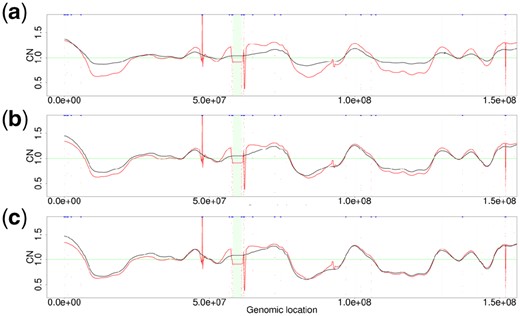
Figure 4 shows an example of the sequential GC corrections and determination of a proper decomposition level for the simulated sequencing data. Initially, CN_Wabico values corrected by means of DOC_GC from decomposition level 1 are calculated [gray line in Fig. 4(a)]. Next, the GC bias in the raw DOC signal is corrected using DOC_GC from decomposition level 2 [black line in Fig. 4(a)]. The curve of CN_Wabico at level 2 is closer to the value 1.0 on the y-axis than that of CN_Wabico at level 1. The y-axis value 1.0 represents an even distribution of CN values regardless of GC proportion in the genomic windows. Here, the direction of changes in CN_Wabico is increasing in genomic windows whose GC proportion is less than 0.4 [white color in the bar of Fig. 4(a)], while that of CN_Wabico is decreasing in genomic windows whose GC proportion is greater than 0.4 [black color in the bar of Fig. 4(a)]. These directions of changes from level 1 to level 2 for all GC windows are the initial directions of changes. Figure 4(b) presents CN_Wabico values corrected with DOC_GC from level 2 (gray curve) to level 3 (black curve). The black color in the bottom bar of Figure 4(b) denotes the GC proportions in which directions of changes are consistent with the initial direction of changes from level 1 to level 2, showing that 90% of the GC proportions are consistent. We continue to decompose until the consistent proportion is less than 50%. Figure 4(d) indicates that the consistent proportion is less than 50% when the decomposition level is greater than 6. Thus, DOC_GC from the level 6 decomposition is finally selected for correcting GC bias in the raw DOC signal [Fig. 4(c)]. Details about the decomposition stopping criteria are provided in Supplementary Figure S3, Figure S4 and Section 1.4.

Fig. 4.

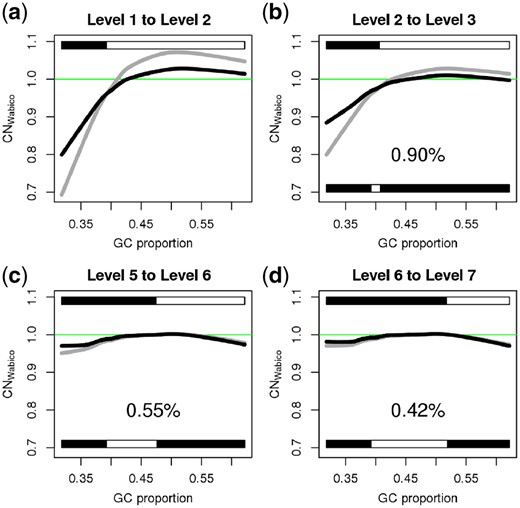
An example of multiresolution GC bias correction. (a) CN_Wabico values from level 1 (gray) to level 2 (black). (b) CN_Wabico values from level 2 (gray) to level 3 (black). (c) CN_Wabico values from level 5 (gray) to level 6 (black). (d) CN_Wabico values from level 6 (gray) to level 7 (black). Upper bars in all the panels show the direction of changes from level i to level i + 1. The black color and white color in these upper bars indicate increasing and decreasing directions, respectively. Bottom bars in panels (b), (c) and (d) denote the ratio of change directions consistent with the initial direction of changes. Black areas represent the proportion consistent with the initial direction of changes. CN_Wabico values on the y-axis are the average of CN_Wabico at 102 400 uniquely mappable positions

2.8 GC bias correction by other methods

We compared the performance of Wabico with that of the following approaches to GC bias correction. The uncorrected CN ratio signal is calculated using the following formula:

$$C{N}_{i,\mathit{raw}}=\frac{\mathit{DO}{C}_{i,\mathit{raw}}}{\mathit{median}(\mathit{DO}{C}_{k,\mathit{raw}})},$$

(3)

where $\mathit{median}(\mathit{DO}{C}_{k,\mathit{raw}})$ is the median of all raw DOCs from the given chromosomes.

In the naive GC correction method, the corrected CN ratio signal is calculated from the GC proportion of the fixed window with a size of 100 bp. It is computed via the following formula:

$$C{N}_{i,\mathit{naive}}=\frac{\mathit{DO}{C}_{i,\mathit{raw}}}{\mathit{mean}(\mathit{DO}{C}_{\mathit{GC}(k)=\mathit{GC}(i),\mathit{raw}})},$$

(4)

where $\mathit{mean}(\mathit{DO}{C}_{\mathit{GC}(k)=\mathit{GC}(i),\mathit{raw}})$ is the average of DOC_raw bins whose GC value is equal to the GC of the ith bin.

The corrected CN ratio signal from the BIC-Seq2-based expected read count is calculated by means of the following formula:

$$C{N}_{i,\mathit{BIC}-\mathit{Seq}2}=\frac{\mathit{DO}{C}_{i,\mathit{raw}}}{\mathit{DO}{C}_{i,\mathit{expected}}},$$

(5)

where $\mathit{DO}{C}_{i,\mathit{expected}}$ is the expected numbers of reads in bin i generated from the BIC-Seq2 normalization step.

3 Results

We applied Wabico to the simulated sequencing reads containing GC bias. We also applied Wabico to the real glioblastoma multiforme (GBM), ovarian cancer (OVC) and lung adenocarcinoma (LUAD) WGS datasets from TCGA. Authorization was obtained from the database of Genotypes and Phenotypes (accession No. phs000178.v8.p7). The real data were generated on the Illumina HiSeq or GenomeAnalyzer platform. All the BAM files are aligned to the hg19 human reference sequence.

For quantifying DOC values of the WGS data, we set a genomic window consisting of 100 uniquely mappable genomic positions, where a 50mer sequence at the position is uniquely aligned to that position but not elsewhere (Xi et al., 2016). In this section, we denoised the CN signals by a TI wavelet transform denoising procedure (Coifman and Donoho, 1995) before investigating GC effects in the CN signals. To get denoised CN signals, we decomposed a CN signal up to decomposition level 15 and set the wavelet denoising parameter C to 2. See Jang et al. (2016) for details of the denoising procedure.

3.1 GC bias correction in simulated data

We used Pysim-sv (Xia et al., 2017) for generating simulated short sequencing reads. Chromosomes 8 and 22 from hg19 were selected for the simulation. First, we created diploid sequences of chromosomes 8 and 22 and then generated 100 bp short reads with 30× coverage. Because Pysim-sv has a function for simulating GC bias, we generated various patterns of GC biases based on the formula $y=-z\times {(x-0.6)}^2+1$ in Pysim-sv, where x represents the GC proportion of the sequencing reads, y denotes a sampling rate and z is a constant value: 2.5 in the original code. Severity of the GC bias increases as z increases. Figure 5(a) presents the results on three z values such as 5 (blue), 20 (purple) and 50 (red). Figure 5(b) shows LOESS-fitted GC bias curves of CN_raw from the sequencing reads for these z values. Figure 5(c) depicts a CN_raw signal representing fluctuations of GC bias for three z values. As z increases, the fluctuation of the signal increases.

Fig. 5.

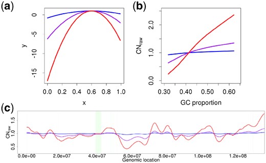
GC bias effects from simulated sequencing reads for various z values. (a) Plots for the GC bias formula at z values of 5 (blue), 20 (purple) and 50 (red), where the x-axis and y-axis represent the x and y values in $y=-z\times {(x-0.6)}^2+1$ in Pysim-sv, respectively. (b) LOESS-fitted GC bias curves of CN_raw for the three z values. CN_raw values on the y-axis are the average of CN_raw at 102 400 uniquely mappable positions. (c) CN_raw at various z values. The green area represents the centromere region of the chromosome in the reference sequence

Figure 6(a, b and c) shows the results of GC bias correction by Wabico for simulated reads with z values of 5, 20 and 50, respectively. Black lines in the plots represent CN_Wabico values. Readers can see that even if GC biases increase severely, the fluctuations of CN_Wabico values decrease effectively.

Fig. 6.

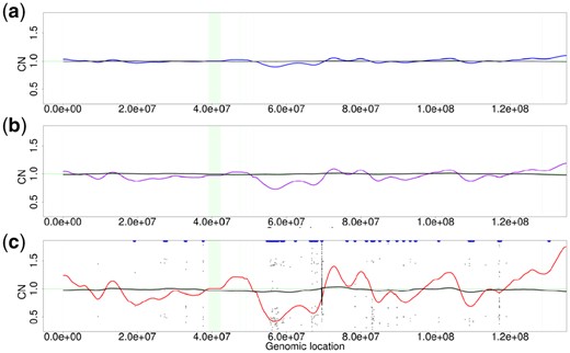
CNs corrected by Wabico. The blue signal in panel (a), the purple signal in (b) and the red signal in (c) are the same signals CN_raw with the corresponding colors in Figure 5 (c). The black signals in (a), (b) and (c) are CN_Wabico for Wabico

We compared other approaches with Wabico: $C{N}_{\mathit{BIC}-\mathit{Seq}2}$⁠, CN_naive and CN_raw. Because the standard deviations (SD) of CN values after GC correction decrease as GC is corrected better, we compared SDs of CN ratios among these four approaches. In Figure 7, blue, green, red and black lines are SDs of CN_raw, CN_naive, $C{N}_{\mathit{BIC}-\mathit{Seq}2}$ and CN_Wabico at various z values. SDs of CN_Wabico values are smaller than those of CN_raw, CN_naive and $C{N}_{\mathit{BIC}-\mathit{Seq}2}$ across various z values, suggesting that Wabico shows more stable correction performance as compared to the other methods. Supplementary Figure S5 presents the comparison of CN_Wabico and $C{N}_{\mathit{BIC}-\mathit{Seq}2}$ when z is 50. CN_Wabico yields smoother results than $C{N}_{\mathit{BIC}-\mathit{Seq}2}$ does. Moreover, we compared the performance of the GC correction methods using the simulated data with CN alterations. We created other simulation data with various levels of GC bias and 10 CN variations that are evenly spaced. CN alterations were identified after GC bias correction by Wabico and BIC-seq2-based expected read count. F1 scores of CN_Wabico were consistently higher than those of $C{N}_{\mathit{BIC}-\mathit{Seq}2}$ at any GC bias severity. Details are shown in Supplementary Figure S6.

Fig. 7.

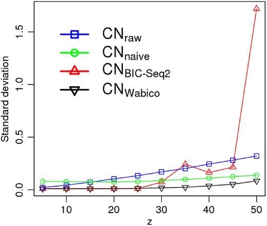
SD of simulated CN ratios at various z values from 5 to 50. Blue, green, red and black lines represent the SDs of denoised CN_raw, CN_naive, $C{N}_{\mathit{BIC}-\mathit{Seq}2}$ and CN_Wabico signals, respectively

In addition, we applied Wabico and BIC-Seq2-based expected read count to the WGS data of paired normal samples of the 37 patients with GBM. When SDs of CN_Wabico and $C{N}_{\mathit{BIC}-\mathit{Seq}2}$ were compared, SDs of CN_Wabico were smaller in 35 samples (Supplementary Table S1).

3.2 GC bias correction of real cancer datasets

Figure 8 shows the results of GC bias correction via multilevel decomposition of chromosome 7 of the TCGA-15-1444-01A sample from GBM. Left-hand plots of Figure 8 depict the denoised CN values, and right-hand plots are GC bias curves of the CN ratio in the 102 400 bp of uniquely mappable genomic positions. Genomic regions within the dotted box indicate the CN alterations around CDK6, which is known as a gene associated with cancer. Figure 8(a) presents CN_raw, and the alteration around CDK6 is not distinguished well from the neighboring signals. In addition, due to the severe fluctuation of the signal across chromosome 7, it incorrectly seems that there are severe CN changes across the chromosome. Figure 8(b) shows the effect of GC correction when CN_Wabico values are obtained by GC bias correction at decomposition level 1. The alteration around CDK6 is more distinguishable than that in Figure 8(a). Although the amplitude of fluctuations decreased, the GC bias still influences the signal. Figure 8(c and d) depicts the results of GC bias correction at decomposition levels 5 and 10. As the decomposition levels increase, the fluctuations decrease significantly and the alterations around CDK6 are more distinguishable.

Fig. 8.

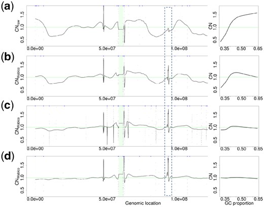
CN signals on chromosome 7 (left) and GC bias curves (right) of sample TCGA-15-1444-01A. CN_Wabico values on the y-axis of the GC bias plots are the average of CN_Wabico at 102 400 uniquely mappable positions. (a) CN_raw values and their GC bias curve. (b) CN_Wabico values and their GC bias curve obtained with DOC_GC constructed from level 1 decomposition. (c) CN_Wabico values and their GC bias curve obtained by means of DOC_GC constructed from level 5 decomposition. (d) CN_Wabico from level 10 decomposition

Figure 9 illustrates how well the GC bias effect embedded in sample TCGA-15-1444-01A is recovered by the fitted coefficients of TI wavelet transform decomposition. In Figure 9(a–c), the denoised CN_raw (red color) is compared with $C{N}_{\mathit{control}}=\frac{\mathit{DO}{C}_{i,\mathit{GC}}}{\mathit{median}(\mathit{DO}{C}_{k,\mathit{GC}})}$ at decomposition levels 1, 5 and 10 (black color), respectively. As decomposition levels increase, the fluctuation patterns of CN_control become more similar to those of CN_raw. Supplementary Figure S7 shows the distribution of CN_Wabico. As decomposition levels increase, the peaks in the distribution become more distinguishable.

Fig. 9.

Similarities of the GC bias pattern between the CN_raw signal and CN_control signal on chromosome 7 of the TCGA-15-1444-01A sample. The red signals in panels (a), (b) and (c) are CN_raw signals in Figure 8(a). The black signals in (a), (b) and (c) are CN_control signals generated at levels 1, 5 and 10, respectively

In our previous study (Jang et al., 2016), we successfully identified focal alterations around known cancer genes in TCGA WGS data after normalizing tumor samples to paired normal samples. In the present study, we tested whether the alterations around these genes can be identified without normal controls if we apply the proposed GC correction method to tumor samples. A cancer gene was considered to be identified if the two conditions in Supplementary Material were satisfied. Tables 1, 2 and 3 list the known cancer genes and the number of samples with alteration in these genes for GBM, LUAD and OVC WGS datasets, respectively. Wabico identified altered cancer genes in most of TCGA samples without normal control data, except for some genes located in regions that are not sufficiently distinguishable as focal aberrations, such as EGFR in the TCGA-06-0686-01A GBM sample and CDK4 in the TCGA-15-1444-01A GBM sample.

Table 1.

CN-altered GBM-related genes

Chr	Start	End	Name	Type	Total	Identified	Ratio
1	204485511	204542871	MDM4	amp	6	6	1.00
4	1795034	1810599	FGFR3	amp	4	4	1.00
4	55095264	55164414	PDGFRA	amp	6	6	1.00
6	163835032	163999628	QKI	del	3	3	1.00
7	55086714	55324313	EGFR	amp	23	22	0.96
7	92234235	92465908	CDK6	amp	4	4	1.00
9	21967751	21995300	CDKN2A	del	14	14	1.00
9	22002902	22009362	CDKN2B	del	13	13	1.00
10	89622870	89731687	PTEN	del	3	3	1.00
10	123237848	123357972	FGFR2	amp	2	2	1.00
12	4382938	4414516	CCND2	amp	2	2	1.00
12	58141510	58149796	CDK4	amp	11	10	0.91
12	69201956	69239214	MDM2	amp	7	7	1.00
17	73314157	73401790	GRB2	amp	2	2	1.00

Note: ‘Start’ and ‘End’ are starting and ending positions of a gene, respectively. ‘Type’ is amplification or deletion of the gene. ‘Total’ is the number of samples that were found to have an alteration around that gene in our previous study. ‘Identified’ is the number of samples that were detected without normal samples in this study. ‘Ratio’ is ‘Identified’ divided by ‘Total’.

Table 2.

CN-altered LUAD-related genes

Chr	Start	End	Name	Type	Total	Identified	Ratio
5	1253262	1295184	TERT	amp	2	2	1.00
5	58264865	59817947	PDE4D	del	3	3	1.00
9	8314246	10612723	PTPRD	del	2	2	1.00
9	21967751	21995300	CDKN2A	del	2	2	1.00
12	69201956	69239214	MDM2	amp	2	2	1.00
19	30302805	30315215	CCNE1	amp	2	2	1.00

Note: ‘Start’, ‘End’, ‘Name’, ‘Type’, ‘Total’, ‘Identified’ and ‘Ratio’ are the same as those described in Table 1.

Table 3.

CN-altered OVC-related genes

Chr	Start	End	Name	Type	Total	Identified	Ratio
1	40361098	40367928	MYCL	amp	7	7	1.00
1	150547032	150552066	MCL1	amp	4	4	1.00
3	168801287	169381406	MECOM	amp	7	7	1.00
4	1723227	1746898	TACC3	amp	5	5	1.00
4	73939093	74124515	ANKRD17	amp	2	2	1.00
5	1253262	1295184	TERT	amp	4	4	1.00
6	19837617	19840915	ID4	amp	4	4	1.00
8	55370495	55373448	SOX17	amp	7	7	1.00
8	128747680	128753674	MYC	amp	16	16	1.00
10	89622870	89731687	PTEN	del	6	6	1.00
11	77811982	77850706	ALG8	amp	6	6	1.00
12	25357723	25403870	KRAS	amp	4	4	1.00
13	48877887	49056122	RB1	del	4	4	1.00
14	21457929	21465189	METTL17	amp	3	3	1.00
17	29421945	29709134	NF1	del	3	3	1.00
19	30302805	30315215	CCNE1	amp	16	16	1.00

Note: ‘Start’, ‘End’, ‘Name’, ‘Type’, ‘Total’, ‘Identified’ and ‘Ratio’ are the same as those described in Table 1.

In addition, we compared GC bias correction by BIC-Seq2-based expected read counts and by Wabico for identification of these known cancer genes with focal aberrations. For this task, we applied these two GC bias correction methods to tumor samples and then segmented them by the BIC-Seq2 segmentation method. The comparison details and results are presented in Supplementary Tables S2, S3 and S4, showing that Wabico outperformed BIC-Seq2-based expected read counts on GBM, but the two methods identified the same number of genes in LUAD and OVC.

3.3 Correlation with SNP array level 3 datasets

We compared CN_Wabico and $C{N}_{\mathit{BIC}-\mathit{Seq}2}$ by calculating correlation coefficients between each of them and the CN ratio from SNP array level 3 data of the same TCGA samples, where denoised CN_Wabico and $C{N}_{\mathit{BIC}-\mathit{Seq}2}$ served for calculating correlation coefficients. Table 4 reveals that the WGS samples corrected by means of Wabico have higher correlation values with SNP array level 3 data than those corrected by the BIC-Seq2 normalization method for GBM, LUAD and OVC WGS datasets. Supplementary Tables S5, S6 and S7 give correlation values for the GBM, LUAD and OVC samples, respectively. We performed the paired t-test for the difference in correlation coefficients for samples of each cancer type. For GBM and LUAD, there were significant differences, but there was no significant difference for OVC, as shown in the last column of Table 4. Moreover, because the correlations were calculated by means of most markers in the whole genome, they were mostly affected by broad CN changes rather than by focal aberrations. Thus, this result implies that broad CN aberrations can be identified more effectively via the correction using Wabico than the correction using the BIC-seq2-based expected read count.

Table 4.

The number of WGS cancer samples having greater correlation coefficients with the Wabico or BIC-Seq2 method

Cancer	Total	Wabico	BIC-Seq2	P-values
GBM	37	30	7	0.010
LUAD	28	24	4	0.023
OVC	47	25	22	0.116

Note: ‘Cancer’ is a cancer type of TCGA WGS datasets. ‘Total’ is the number of cancer patients in the dataset. ‘Wabico’ is the number of patients with a greater correlation coefficient between SNP level 3 segment and denoised CN values corrected by Wabico than that between SNP array level 3 segment and denoised CN values corrected by BIC-Seq2-based expected read counts. ‘BIC-Seq2’ is the case opposite to ‘Wabico’. ‘P-values’ are obtained by a paired t-test.

In addition, for a further comparison, we applied a CN segmentation method to WGS data that are GC-corrected by Wabico and BIC-Seq2-based expected read counts, and then measured the precision, recall and F1-scores of CN segments by comparing them with CN segments in SNP array level 3 data. F1-scores of CN segments corrected by Wabico were higher than those corrected by the BIC-Seq2-based expected read count in greater numbers of samples for all three tumor datasets. Detailed results are given in Supplementary Tables S8, S9 and S10.

4 Discussion

We developed a new GC bias correction method. We decomposed original DOC into scaling and wavelet coefficients and fitted each coefficient by LOESS regression and kernel smoothing, respectively. After generating DOC_GC, we reduced the GC bias by dividing original DOC by DOC_GC.

We employed variable-size windows for quantifying the mapped reads as BIC-Seq2 did. It has an advantage of reducing the effect of mappability bias by taking into account only uniquely mappable positions. In the wavelet decomposition, we calculated differences and averages of two neighboring genomic regions although their actual genomic lengths could be different. When we set the windows to contain 100 uniquely mappable positions, most of window sizes were 100 bp in hg19. When we manually inspected already known alterations, the effect of variable-size windows did not seem to be substantial.

In Wabico, we used a multiresolution approach to control GC bias. At a given decomposition level, DOC_GC is calculated from GC bias information from the lowest level to that level. Note that the degree of uncertainty in the DOC_GC signal can change according to the decomposition level. As illustrated in Figure 8(c and d), deletion events in Figure 8(c) are removed in Figure 8(d). As the level increases, some false positive events can be removed although true events might be removed as well. Thus, the choice of proper decomposition levels is important. Therefore, in this study, we set the minimal ratio of the direction of changes to the value consistent with the initial direction of changes, 50%. As we increase decomposition levels, consistency values with the initial direction of changes decrease overall (Fig. 4). When the ratios of the consistency fall below 50% at some levels, the plots of DOC_GC for these levels seem to be distorted and do not appear to properly reflect the GC bias embedded in raw input DOC signals. Although this is not a mathematically rigorous decomposition stopping criterion, it works practically well for both simulated and real WGS datasets.

We applied Wabico to the three WGS different tumor types. In the GBM and LUAD data, the WGS samples corrected by Wabico showed significantly higher correlation with SNP array level 3 data than those corrected by the BIC-Seq2 expected read count method while the difference between two methods was marginal in the OVC data. This different result depending on cancer type might be due to other factors in addition to the severity of GC bias. For example, we observed that in the given WGS datasets, the OVC samples are CN altered in more genomic regions than the GBM and LUAD samples. Thus, more research is required to investigate the effect of other factors such as cancer characteristics for detecting the CN alterations.

CNVkit (Talevich et al., 2016) is a tool for identification of CN variations in whole-exome sequencing data and provides correction of GC bias in whole-exome sequencing data. To correct GC bias, it employs a rolling median. Those authors reported that on sample data, the rolling median and the LOESS method produced similar fits. Because our method involves the LOESS regression based on multiresolution decomposition, we compared the performances between Wabico and the GC correction method used in the CNVkit method. Wabico showed better performance for all the three tumor types. Comparison details are described in Supplementary Tables S11, S12 and S13 and Figure S8.

Wabico helps to visually inspect fluctuations of the DOC signal that can be checked by GC bias (Figs 5c, 6, 8 and 9]. Furthermore, the DOC values corrected by Wabico can serve as input to segmentation algorithms such as BIC-Seq2 and circular binary segmentation (Olshen et al., 2004) for identifying the exact breakpoint of a CN alteration or for determining integer CNs of genomic regions.

Funding

This work has been supported by a National Research Foundation of Korea (NRF) grant funded by the Korea government (NRF-2016R1A2B2013855), the Bio & Medical Technology Development Program of NRF funded by the Korean government (MSIT) (NRF-2018M3C7A1054935) and GIST Research Institute (GRI) grant funded by the GIST in 2018.