Significance tests for analyzing gene expression data with small sample sizes

Abstract

Motivation

Under two biologically different conditions, we are often interested in identifying differentially expressed genes. It is usually the case that the assumption of equal variances on the two groups is violated for many genes where a large number of them are required to be filtered or ranked. In these cases, exact tests are unavailable and the Welch’s approximate test is most reliable one. The Welch’s test involves two layers of approximations: approximating the distribution of the statistic by a t-distribution, which in turn depends on approximate degrees of freedom. This study attempts to improve upon Welch’s approximate test by avoiding one layer of approximation.

Results

We introduce a new distribution that generalizes the t-distribution and propose a Monte Carlo based test that uses only one layer of approximation for statistical inferences. Experimental results based on extensive simulation studies show that the Monte Carol based tests enhance the statistical power and performs better than Welch’s t-approximation, especially when the equal variance assumption is not met and the sample size of the sample with a larger variance is smaller. We analyzed two gene-expression datasets, namely the childhood acute lymphoblastic leukemia gene-expression dataset with 22 283 genes and Golden Spike dataset produced by a controlled experiment with 13 966 genes. The new test identified additional genes of interest in both datasets. Some of these genes have been proven to play important roles in medical literature.

Availability and implementation

R scripts and the R package mcBFtest is available in CRAN and to reproduce all reported results are available at the GitHub repository, https://github.com/iullah1980/MCTcodes.

Supplementary information

Supplementary data is available at Bioinformatics online.

1 Introduction

Informative feature selection in a noisy high-dimensional covariate space is a commonplace for data scientists and statisticians. One way that this can be achieved is to impose sparsity and use penalized optimization methods, in the same manner as Lasso (Tibshirani, 1996) to obtain a sparse vector of estimated regression coefficients. Another approach is to apply an appropriate univariate two-sample test independently to a large number of features in high-dimensional data in order to select genes that are differentially expressed under two biologically different conditions (Saeys et al., 2007). This is done as a preliminary step to reduce the noise in an ultra-high-dimensional dataset, and it results in a superset that contains the most important features and can be included in a multivariate model for group comparison (Troyanskaya et al., 2002) or cancer subtype identification for chemotherapy (Yeoh et al. 2002. The latter strategy is sometime used for feature discoveries followed by a necessary correction for multiple testing (Beasley et al., 2004; Krzywinski and Altman, 2014b).

In this study, we focus on the second approach of filtering a set of features. Suppose independent samples are collected from two normally distributed populations to test if the two underlying means are the same. This problem is prevalent and is so fundamental that it is introduced in most undergraduate textbooks. While the use of two-sample tests in one form or another continues to be used in a wide variety of research studies, it is not uncommon to observe its incorrect usage. However, the aim of the current study is to improve upon the traditional procedures, while also making use of the computational power bestowed upon us by modern technology.

The Student’s t-test is a more appropriate univariate two-sample test and can be used for filtering purposes. However, it becomes less reliable when there are a limited number of observations and the objective is to filter a large number of variables, with the result that many of them might not meet the equal variance assumption of the test (Krzywinski and Altman, 2014a). Therefore, the Welch’s t-test is rather more common in practice for filtering purposes because it accounts for unequal variances (for example, see Comin et al., 2014; Cui et al., 2010; Yang et al., 2017). The Welch’s test relies on two layers of approximations: approximating the distribution of the statistic by the t-distribution, which in turn depends on the approximate degrees of freedom. In this paper, we use Monte Carlo test (MCT) which uses only one layer of approximation, with the expectation that it will be more reliable than the Welch’s test.

The remainder of this paper is presented as follows. In Section 2, we introduce the proposed test. The test is evaluated using simulation studies in Section 3 and it is applied to childhood acute lymphoblastic leukemia gene expression data in Section 4. We conclude with a discussion in Section 5.

2 Materials and methods

We begin with the necessary notation, as well as various versions of the test that are taught in elementary schools and are widely used in practice. Suppose that data $(x_1,x_2,\dots ,x_m)$ and $(y_1,y_2,\dots ,y_n)$ are generated from $N(\mu ,{\sigma }_x^2)$ and $N(\mu +\delta ,{\sigma }_y^2)$⁠, respectively. Let $\overline{x}={\sum }_{i=1}^m{x}_i/m$ and $\overline{y}={\sum }_{i=1}^n{y}_i/n$ be the sufficient statistics (when ${\sigma }_x^2$ and ${\sigma }_y^2$ are known), and the observed difference $\overline{x}-\overline{y}$ follows a normal distribution with mean δ and variance ${\sigma }_x^2/m+{\sigma }_y^2/n$ i.e. $\overline{x}-\overline{y}\sim N(\delta ,{\sigma }_x^2/m+{\sigma }_y^2/n)$⁠. To test the null hypothesis $H_0:\delta =0$⁠, a number of approaches can be used depending on the underlying assumptions. We here build up on some well-known approaches.

When ${\sigma }_x^2$ and ${\sigma }_y^2$ are given, then under H₀, a uniformly most powerful (UMP) test exists, which is widely recognized as z-test in the literature. To perform the test, define

$$Z=\frac{\overline{x}-\overline{y}-\delta }{\sqrt{\frac{{\sigma }_x^2}{m}+\frac{{\sigma }_y^2}{n}}}.$$

(1)

The quantity Z is pivotal (see Casella and Berger, 2002) and it follows a standard normal distribution under the null hypothesis (δ = 0). A larger observed value of the magnitude of Z supports the evidence against the null hypothesis.

Suppose that, rather than the two variances, only their ratio, $\rho ={\sigma }_y^2/{\sigma }_x^2$⁠, is known, then one can obtain a ‘pooled’ estimator of ${\sigma }_x^2$ as

$${\widehat{\sigma }}_x^2=\frac{(m-1)s_x^2+(n-1)s_y^2/\rho }{(m+n-2)},$$

(2)

where $s_x^2={\sum }_{j=1}^m{(x_i-\overline{x})}^2/(m-1)$ and $s_y^2={\sum }_{j=1}^n{(y_i-\overline{y})}^2/(n-1)$ are the sufficient statistics.

Here the variance information from the y group is also used in estimating ${\sigma }_x^2$ because $s_y^2/\rho$ also has the expectation ${\sigma }_x^2$⁠. In this case, the estimator of ${\sigma }_y^2$ is ${\widehat{\sigma }}_y^2=\rho {\widehat{\sigma }}_x^2$⁠. Replacing the two unknown parameters in (1) by their estimators ${\widehat{\sigma }}_x^2$ and ${\widehat{\sigma }}_y^2$ produces the following pivotal statistic:

$$T_p=\frac{\overline{x}-\overline{y}-\delta }{\sqrt{\frac{{\widehat{\sigma }}_x^2}{m}+\frac{{\widehat{\sigma }}_y^2}{n}}}.$$

(3)

In fact, the distribution of T_p is known and is exactly a t-distribution with $(m+n-2)$ degrees of freedom. Note that a special case exists when ρ = 1 (i.e. ${\sigma }_x^2={\sigma }_y^2$⁠), T_p is recognized as the Student’s t-test. As is apparent, the Student’s t-test is valid and exact as long as the true variance ratio ρ is known (even if the two variances are not equal).

To proceed, let us first recall that a random variable following a t-distribution with degree of freedom d can be expressed as

$$\frac{Z}{\sqrt{\mathcal{D}}},$$

where Z and $\mathcal{D}$ are two independent random variables, $Z\sim N(0,1)$ and $\mathcal{D}$ is a scaled χ² distribution with a unit mean, ${\chi }^2(d)/d$⁠. We now introduce an extended t-distribution with the parameters λ, d₁ and d₂ given by

$$T_G=\frac{Z}{\sqrt{\mathcal{D}}},$$

in which $\mathcal{D}$ is replaced by a sum of two scaled χ² distributions, $\lambda \hspace{0.17em}{\chi }^2(d_1)/d_1+(1-\lambda )\hspace{0.17em}{\chi }^2(d_2)/d_2$⁠. The exact density function can be obtained by the combination proportion λ and two parameters for the degrees of freedom (d₁, d₂). We will denote its distribution as $t_g(\lambda ,d_1,d_2)$⁠. In certain cases, when λ = 0 or 1, or d₁ = d₂, this extended t_g becomes the traditional t-distribution.

In practice, however, the variance values and their ratios ρ are commonly unknown. Therefore, we do not have a pivotal statistic whose exact distribution is known. This leads us to the fact that no UMP test exists in the literature. Different variance estimators of $\overline{x}-\overline{y}$ produces different test statistics. Consider the well-known statistic

$$T=\frac{\overline{x}-\overline{y}-\delta }{\sqrt{\frac{s_x^2}{m}+\frac{s_y^2}{n}}}.$$

(4)

The quantity T in (4) is asymptotically normally distributed with a mean of 0 and a variance of 1 when δ = 0. Thus, both m and n are required to be sufficiently large so that ${\sigma }_x^2$ and ${\sigma }_y^2$ can be well approximated by $s_x^2$ and $s_y^2$⁠, and T becomes equivalent to $Z\sim N(0,1)$⁠. However, unlike Z and T_p, the exact distribution of T is generally unknown.

To this end, the approximate distribution for T is of great interest, especially when the sample sizes m and n are small. A reasonable approximation specifies a critical value for the test to meet the nominal level (e.g. $\alpha =0.05$⁠). Ideally, the critical values should be chosen so that the test is unbiased (i.e. false positive rate also known as size of the test is as specified). The statistic in (4) does not meet this criterion when normal approximation is used and is highly liberal unless the sample sizes are very large.

In cases where the sample sizes are small and the two variances are close (⁠$\rho \approx 1$⁠), the Student’s t-test (the statistic T_p with student t-distribution approximation) not only holds the nominal level, but it is also powerful and therefore recommended. However, in cases when the assumption of the equal variances cannot be met or, more broadly speaking, the ratio ${\sigma }_x^2/{\sigma }_y^2$ is unknown, the Student’s t-distribution becomes an approximation to the true distribution of T. Furthermore, the approximation relies on the best ‘matched’ degree of freedom for the t-distribution.

The test problem is known as the Behrens–Fisher (BF) problem when no assumption of equal population variances can be made. For the BF problem, the T statistic provides value for a given dataset and its statistical distribution is not easy to characterize. More formally, the P-value cannot be calculated exactly under the null unless $\tau =({\sigma }_x^2/m)/({\sigma }_y^2/n)$ is specified. This results in a number of approximate tests (for example, see Best and Rayner, 1987; Fenstad, 1983; Welch, 1938). To our knowledge, the best approximation thus far is due to Welch (1938). Note that it is not recommended to pre-test the ρ values (e.g. ρ = 1) and then choose between the Student’s t-test and the Welch’s approximate t-test. Rather, the Welch’s t-test can be applied directly.

In reality, if we do not know the true values of the underlying variances (or ρ), there exists an entire family of distributions in which only one is the true distribution of T. It is important to note that the Welch’s test first chooses a t-distribution as an approximation to the distribution of T whose degrees of freedom are then estimated from the available data. When τ takes values 0 and $\infty$⁠, the approximation becomes exact under the null and the statistic T follows an exact t-distribution with the degree of freedom being m − 1 and n − 1, respectively.

As described in the next section, we avoid one layer of approximation while making use of the Monte Carlo simulations from the exact distributions. This gives us an apparent advantage over Welch’s t-approximation.

2.1 Monte Carlo solutions

The statistic in (4) can be re-expressed as

$$T=\frac{\frac{\overline{y}-\overline{x}-\delta }{\sqrt{{\sigma }_x^2/m+{\sigma }_y^2/n}}}{\sqrt{\frac{s_x^2/m+s_y^2/n}{{\sigma }_x^2/m+{\sigma }_y^2/n}}}=\frac{Z}{\sqrt{\mathcal{D}}}.$$

Here $Z\sim N(0,1)$ when δ = 0 as described in the previous section. Clearly $\mathcal{D}$ is a convex combination of ${\chi }_{(m-1)}^2/(m-1)$ and ${\chi }_{(n-1)}^2/(n-1)$ (Welch, 1938),

$$\mathcal{D}=\frac{s_x^2/m+s_y^2/n}{{\sigma }_x^2/m+{\sigma }_y^2/n}$$

$$\sim \frac{\frac{{\chi }_{(m-1)}^2}{m-1}\frac{{\sigma }_x^2}{m}+\frac{{\chi }_{(n-1)}^2}{n-1}\frac{{\sigma }_y^2}{n}}{{\sigma }_x^2/m+{\sigma }_y^2/n}$$

$$\sim \lambda {\kappa }_1+(1-\lambda ){\kappa }_2$$

where ${\kappa }_1\sim {\chi }_{m-1}^2/(m-1),\hspace{0.17em}{\kappa }_2\sim {\chi }_{(n-1)}^2/(n-1)$ and $\lambda =({\sigma }_x^2/m)/({\sigma }_x^2/m+{\sigma }_y^2/n)=n/(n+\rho m)$⁠. Therefore, the T statistic follows an extended t-distribution $t_G(\lambda ,n_1-1,n_2-1)$⁠. If we know λ, the distribution of $\mathcal{D}$ can be easily generated via simulations, as analytical expressions are too cumbersome to be of much use in this case.

In the absence of computers, as was the case 70 years ago, Welch (1938) approximated $\mathcal{D}$ by a gamma distribution (scaled χ² distribution) by matching the first two moments. This leads to the t-distribution approximation for T with a degree of freedom as

$$f=\frac{{\left(\frac{{\sigma }_x^2}{m}+\frac{{\sigma }_y^2}{n}\right)}^2}{\frac{{\sigma }_x^4}{m^2\left(m-1\right)}+\frac{{\sigma }_y^4}{n^2\left(n-1\right)}},$$

which depends on the values of the variances (via $\rho ={\sigma }_y^2/{\sigma }_x^2$⁠). Of course, if we knew the variance values, or even just the ratio, we would be able to use the z-test or the exact t-test given by (1) or (3), respectively, and there would not be a need for the t-distribution approximation. In practice, we would estimate f by substituting the corresponding sample variances into unknown variances, and the distribution of T would be approximated by the t-distribution with the data-dependent degree of freedom,

$$\widehat{f}=\frac{{\left(\frac{s_x^2}{m}+\frac{s_y^2}{n}\right)}^2}{\frac{s_x^4}{m^2\left(m-1\right)}+\frac{s_y^4}{n^2\left(n-1\right)}}.$$

(5)

The t-test therefore relies on two layers of approximation: firstly, the t-distribution itself and secondly, the ‘best’ degree of freedom estimated by (5). Realizing $\widehat{f}$ above is subject to uncertainty, Barnard (1984) listed exact P-values for the T statistic for a range of possible variance ratio ρ values and then averaged them to obtain the final P-value.

The t-approximation essentially uses a single χ² distribution for $\mathcal{D}$ that has a mixture of two χ² distributions. An alternative approach, therefore, is to simply find the most appropriate mixing parameter $\tilde{\lambda }$ so that $\tilde{\mathcal{D}}\sim \tilde{\lambda }{\kappa }_1+(1-\tilde{\lambda }){\kappa }_2$ is a good approximation to $\mathcal{D}$ in some sense (e.g. matching the mean and the variance). One possibility is to substitute the corresponding sample variances into an unknown variance ratio as an estimate of the ratio, $\widehat{\rho }=s_y^2/s_x^2$ and obtain

$$\widehat{\lambda }=\frac{n}{n+\widehat{\rho }m}.$$

(6)

Once the distribution of $\mathcal{D}$ is in place, the distribution of T can be easily generated from $Z/\sqrt{\mathcal{D}}$⁠. For example, in R, we can easily generate 100 000 random numbers from $Z/\sqrt{\tilde{\mathcal{D}}}$⁠.

> MC <-100000

> lam <- (var(X[, 1])/n1)/(var(X[, 1])/

+ n1+var(Y[, 1])/n2)

> MC.T <- rnorm(MC)/sqrt(lam*rchisq(MC, n1-1)

+ /(n1-1) + n(1-lam)*rchisq(MC, n2-1)/(n2-1))

The corresponding P-value can then be obtained by counting how many MC.T values exceed the observed T value. For a two-sided test, the P-value is obtained using the following codes:

> p.value = mean(abs(MC.T) >= abs(obs.T))

We denote this Monte Carlo procedure by MCT.

3 Numerical results

To see how the proposed approximation performs, we conducted simulation studies. In these simulation studies, we compared the new MCT with the Welch’s t-test (henceforth denoted by W) to determine if any improvement exists.

We considered various sample size combinations that reflected small to large sample sizes and different variance ratios. For sample sizes m and n we considered 4, 5, 8, 10, 25 and variance ratios varying from $2^{-8}$ to 2⁸. Note that the values of τ are determined from the values of ${\sigma }_x^2,\hspace{0.17em}{\sigma }_y^2$⁠, m and n. Following Best and Rayner (1987), the shift parameter δ, which measure the deviation from the equality of means, was obtained by $\delta =\eta \sqrt{{\sigma }_x^2/m+{\sigma }_y^2/n}$⁠, where η is an appropriate constant. For the false positive rate comparison, we used η = 0, while for a power comparison we used $\eta =1,2,3$⁠. The empirical size results are provided in Supplementary Tables S1–S6 and the empirical power results are given in Supplementary Tables S7–S12.

Based on the simulation results, it is apparent that the level performance of the two procedures are almost the same and that they hold the nominal level reasonably well. The power of the MCT is, in general, better than that of the W, especially when the sample with a smaller sample size has the larger variance (Fig. 1).

Fig. 1.

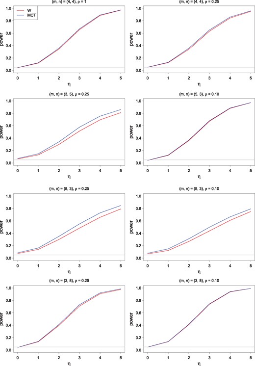
Empirical size (false positive rate) and power of W and MCT as a function of η. A gray horizontal line in each panel indicates the nominal size $\alpha =0.05$

Next, we compared the densities of the Welch’s approximate t-distribution and the Monte Carlo approximation to the true distribution of T (Monte Carlo is based on true λ). In particular, we targeted the scenarios where the MCT and W differed, and the use of MCT became clearly advantageous (i.e. when the m and n are small, different and the sample with a smaller sample size has the larger variance). For example, we took m = 6, n = 3, ${\mu }_x={\mu }_y=1,\hspace{0.17em}{\sigma }_x^2=1,\hspace{0.17em}{\sigma }_y^2=1.44$⁠. The densities are depicted in Figure 2. The Figure shows that the Welch’s approximate t-distribution tailed off more slowly than the Monte Carlo approximation, which was also closer to the true distribution of T. This shows that the MCT is more powerful than the W.

Fig. 2.

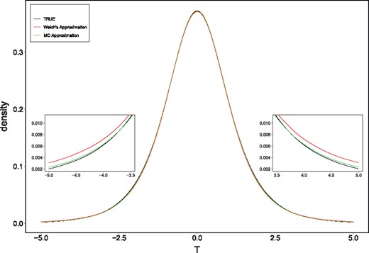
Plot of the true density of T overlaid with the t-distribution using the Welch approximate degrees of freedom and the Monte Carlo approximation based on $\widehat{\lambda }$⁠; m = 6, n = 3, ${\mu }_x={\mu }_y=1,\hspace{0.17em}{\sigma }_x^2=1,\hspace{0.17em}{\sigma }_y^2=1.44$⁠. The tails are magnified to see the differences between the different approximations more clearly

We further investigated the effect of changes in sample sizes on the two approximations relative to the true distribution of T. We considered m = 8, $n_2=3,5,7,\hspace{0.17em}{\mu }_x={\mu }_y=1,\hspace{0.17em}{\sigma }_x^2=1$ and ${\sigma }_y^2=2.25$⁠. Table 1 shows the quantiles of the distributions. As Table 1 suggests, the quantiles of the Monte Carlo approximation were much closer to the quantiles of the true density as compared to the Welch approximation, especially when n₂ was small. As n₂ was increased, the Welch’s approximation became closer to the true density, but the MC approximation still appeared to be better.

Table 1.

The quantiles of true density of T based on λ (⁠${\text{MC}}_{\lambda }$⁠), the t-distribution using the Welch approximate degrees of freedom (W) and the Monte Carlo approximate distribution based on $\widehat{\lambda }$ (⁠${\text{MC}}_{\widehat{\lambda }}$⁠); m = 8, ${\mu }_x={\mu }_y=1,\hspace{0.17em}{\sigma }_x^2=1,\hspace{0.17em}{\sigma }_y^2=2.25$

		Quantile
Method	n	1%	5%	10%	90%	95%	99%
${\text{MC}}_{\lambda }$		−3.878	−2.270	−1.619	1.618	2.270	3.881
W	3	−4.639	−2.356	−1.634	1.635	2.356	4.637
${\text{MC}}_{\widehat{\lambda }}$		−3.831	−2.221	−1.587	1.587	2.222	3.831
${\text{MC}}_{\lambda }$		−2.981	−1.903	−1.422	1.422	1.903	2.980
W	5	−3.072	−1.918	−1.426	1.426	1.918	3.073
${\text{MC}}_{\widehat{\lambda }}$		−2.977	−1.897	−1.418	1.418	1.897	2.977
${\text{MC}}_{\lambda }$		−2.726	−1.802	−1.367	1.367	1.802	2.725
W	7	−2.768	−1.813	−1.372	1.373	1.813	2.768
${\text{MC}}_{\widehat{\lambda }}$		−2.743	−1.808	−1.370	1.370	1.808	2.743

To see the robustness of the MCT against the assumption of normality, we simulated data from a t-distribution with 5 degrees of freedom, $t_{(5)}$⁠. The empirical false positive rate and power tables are diverted to supplementary materials (Supplementary Tables S13–S16). Supplementary Table S13 shows the simulation results using $t_{(5)}$ errors. It appears that the MCT is slightly better or at least as robust as the W against deviations from normality both in terms of false positive rate and power. For example, the average empirical false positive rates (over the 45 scenarios) were equal to 0.9% for both methods at 1% nominal level. However, at 5 and 10% nominal levels, the average false positive rates were, respectively, 4.5 and 9.4% for W while these were, respectively, 4.6 and 9.6% for MCT. However, larger studies would be required to further validate this claim, which we aim to carry out using very different distributions including more heavy tailed and skewed distributions.

4 Applications

4.1 Analysis of the Golden Spike dataset

To provide additional evidence of the superior performance of the MCT over the W, we applied both tests to a real dataset known as Golden Spike dataset (Choe et al., 2005). The dataset is produced by a controlled experiment and the true differentially expressed genes (DEGs) are known. As a result, it has been used for the benchmarking of the microarray analysis methods (for example, see Hochreiter et al., 2006; Roca et al., 2017, and references therein).

This dataset includes two experimental groups, namely control and spike-in, with three technical replicates per group. As is described in Hochreiter et al. (2006), the dataset has 13 966 probe sets. The number of differentially spiked-in probe sets were 3876 (excluding Affymetrix internal control probes). Out of these 3876 spiked-in probe sets, 1328 were spiked-in at higher concentrations in the spiked-in group at a fold-change level of interest that ranged from 1.1- to 4.0-fold between the two groups, 2535 were spiked-in at the same concentration in both groups, and the remaining probe sets had weak matching to multiple clones (Hochreiter et al., 2006).

We did the background correction using the Affymetrix MAS5 algorithm implemented in the mas5 function of the affy package (Gautier et al., 2004). A probe set that was not called present by the MAS5 algorithm was considered as missing. We excluded the missing probe sets and the Affymetrix control probe sets from the remainder of the analysis. The data were then normalized using SVCD normalization, which is proven to be superior by Hochreiter et al. (2006).

We applied the W and MCT tests to the processed data and the P-values that were obtained were adjusted via the ‘fdr’ method (Benjamini and Hochberg, 1995) implemented in the p.adjust() function of the stats package. The adjusted P-values for the W and MCT are presented in Figure 3. The MCT produced smaller P-values for the known positives (true differentially expressed probes) than those that were produced by W, which proves that the MCT is more powerful. In addition, the P-values of the MCT for the known negatives were larger than the P-values of the W, hence reducing a type-1 error. At a 1% significance level, the W detected 555 genes (527 and 15 were from the differently expressed spiked-in group and control group, respectively) while our MCT detected 744 genes (691 and 21 were from the differently expressed spiked-in group and control group, respectively). The corresponding false positive rate for the W was 0.74%, which was quite different from the nominal 1% level. Our MCT, on the other hand, produced a much more accurate value of 1.04%. Next, we increased the nominal significance level so that the W produced a false positive rate close to 1%, and we determined that the corresponding true detection rate increased from 41.5% (527/1271) to 51.8% (658/1271). Note that the true detection rate for our MCT was 54.1% (688/1271), which is higher than the adjusted detection rate of W (51.8%).

Fig. 3.

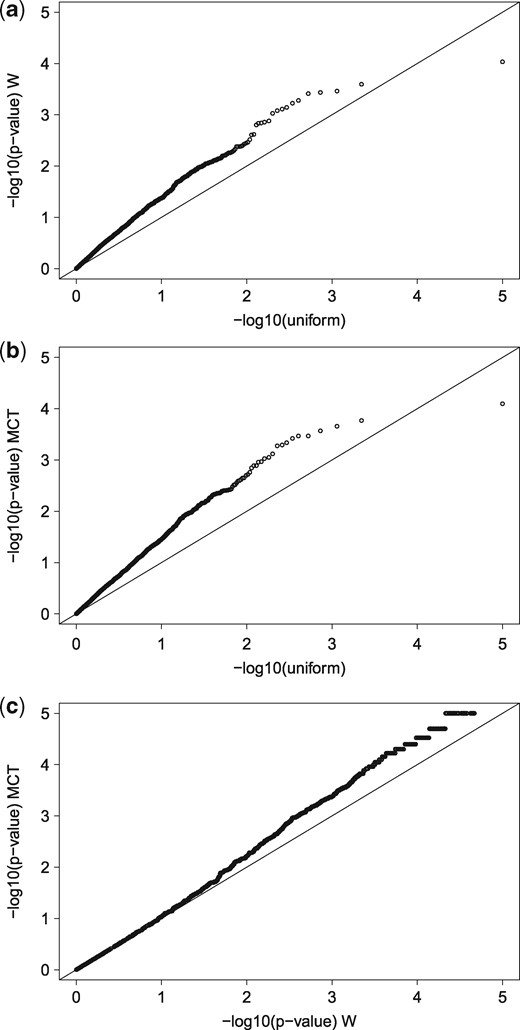
QQ-plots of the P-values obtained via W and MCT. In (a) and (b), the P-values for known negative probes were obtained via W and MCT, respectively, and they were plotted against a standard uniform variate on −log10 scale. In (c), the P-values for known positive probes were obtained via W and are plotted against those obtained via MCT on −log10 scale

4.2 Childhood acute lymphoblastic leukemia gene expression study

To show the benefits of the MCT, we chose a childhood acute lymphoblastic leukemia (ALL) high-throughput gene-expression dataset that is studied in detail by Den Boer et al. (2009) and accessible through GEO Series accession number GSE13425. The data had 22 283 genes and 190 samples in total. The 190 samples are from different subtypes of ALL. We considered only two ALL subtypes: BCR-ABL, which has four samples and E2A-rearranged (EP), which has eight samples. This is because under small and different sample sizes, the difference between the MCT and W is more pronounced and we expected the MCT to produce favorable results in situations where a large number of tests are performed to identify variables that can possibly be used to classify two the groups. Under a large sample size, however, the performance of the two tests is similar.

We did the background correction using the Affymetrix MAS5 algorithm implemented in the limma package (Ritchie et al., 2015). A probe set that was not called present for at least two samples in each subtype by the MAS5 algorithm was considered as missing. We excluded the missing probe sets and the Affymetrix control probe sets from the rest of the analysis. This process drops the number of genes from 22 283 to 6307. These 6307 genes were then normalized using MedianCD normalization (SVCD did not converge in 200 iterations) also proposed by Hochreiter et al. (2006), and this appeared to have almost comparable performance to SVCD.

We applied the W and MCT tests to the processed genes. Based on the P-values, the W test found 586 (1478) probes differentially expressed at a 0.01 (0.05) level of significance between BCR-ABL and E2A-rearranged (EP) ALL patients. The MCT test, on the other hand, detected 72 (56) additional DEGs and it did not miss any of the genes that were identified by the W. A summary of these tests for 72 additional genes is provided in Table 2. As a visual cross-check, we performed a principal component analysis (PCA)—a standard dimension reduction technique in high-dimensional setting—on all of the 6307 probe sets. Figure 4a shows the 12 samples projected onto the first two principal components. The two subtypes are separated into two groups by the second principal component. We repeated PCA, this time taking into account only the 72 genes—namely those that were made significant by the MCT test. Again, the 12 samples are projected onto the first two principal components in Figure 4b. The plot clearly demonstrates that the additional genes identified by the MCT test have the ability to classify the two subtypes.

Fig. 4.

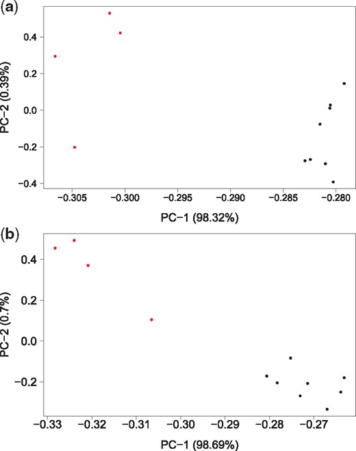
PCA plot of the childhood acute lymphoblastic leukemia (ALL) gene-expression dataset based on (a) all 6307 genes (b) only 72 additional genes identified by the MCT test. The red dots represent subtype BCR-ABL and the black dots represent subtype E2A-rearranged (EP)

Table 2.

The list of 72 additional genes identified by MCT at 0.01 level of significance based on P-values for childhood acute lymphoblastic leukemia gene expression study

	BCR-ABL	E2A-rearranged (EP)	P-values
Probe set ID	Mean (SD)	Mean (SD)	MCT	Welch
NONO$|$200057_s_at	8.58 (0.21)	8.12 (0.2)	0.0085	0.0118
TMED2$|$200087_s_at	7.18 (0.24)	6.64 (0.29)	0.0083	0.0102
CALM$|$200655_s_at	7.83 (0.38)	6.95 (0.17)	0.0089	0.014
LAPTM4A$|$200673_at	7.7 (0.41)	6.83 (0.39)	0.0086	0.0123
PGK1$|$200737_at	5.76 (0.34)	5.01 (0.31)	0.008	0.0116
ARL6IP5$|$200761_s_at	5.67 (0.63)	4.36 (0.6)	0.0098	0.0142
ZNF207$|$200828_s_at	7.93 (0.44)	7 (0.34)	0.0093	0.0141
IST1$|$200851_s_at	7.17 (0.41)	6.28 (0.46)	0.0092	0.012
PSAP$|$200866_s_at	6.58 (0.74)	4.82 (0.42)	0.0064	0.0114
ACTR3$|$200996_at	6.34 (0.42)	5.36 (0.3)	0.0063	0.011
PSMF1$|$201052_s_at	4.78 (0.42)	3.89 (0.47)	0.0096	0.0128
ATP6V1B2$|$201089_at	5.5 (0.59)	4.15 (0.29)	0.009	0.0142
HNRNPH2$|$201132_at	3.8 (0.44)	2.83 (0.51)	0.0095	0.0111
BHLHE40$|$201170_s_at	7.25 (0.99)	4.97 (0.57)	0.0072	0.0129
SEC11A$|$201290_at	6.04 (0.37)	5.18 (0.27)	0.0061	0.0103
SLC9A3R1$|$201349_at	5.33 (0.72)	3.75 (0.55)	0.0084	0.0125
CUL3$|$201371_s_at	7.3 (0.43)	6.32 (0.57)	0.0087	0.0101
ITGA5$|$201389_at	6.04 (0.77)	4.28 (0.58)	0.0062	0.0107
TRAM1$|$201398_s_at	6.59 (0.32)	5.9 (0.36)	0.0096	0.0123
PLEKHB2$|$201411_s_at	5.02 (0.68)	3.18 (1.33)	0.01	0.0101
ETF1$|$201573_s_at	5.92 (0.44)	4.89 (0.22)	0.007	0.0127
IRAK1$|$201587_s_at	6.84 (0.59)	5.58 (0.49)	0.0084	0.013
USP14$|$201672_s_at	6.14 (0.41)	5.2 (0.21)	0.0082	0.0141
EFCAB14$|$201778_s_at	4.68 (0.33)	3.93 (0.44)	0.0097	0.0109
SEC63$|$201914_s_at	4.8 (0.42)	3.86 (0.4)	0.0076	0.0109
SLC25A36$|$201917_s_at	5.72 (0.51)	4.56 (0.26)	0.0078	0.0139
KIF5B$|$201991_s_at	6.23 (0.26)	5.65 (0.22)	0.0068	0.0105
SPG7$|$202104_s_at	3.81 (0.37)	3 (0.41)	0.0089	0.0114
RAP1A$|$202362_at	5.24 (0.63)	3.71 (0.39)	0.005	0.0101
BASP1$|$202391_at	4.45 (0.64)	5.86 (0.78)	0.0094	0.0114
SEC24B$|$202798_at	5.4 (0.59)	4.15 (0.49)	0.0096	0.014
CYTH1$|$202879_s_at	4.86 (0.6)	3.57 (0.52)	0.0094	0.0133
RHOBTB3$|$202975_s_at	3.51 (0.39)	2.66 (0.32)	0.008	0.0125
RREB1$|$203704_s_at	5.44 (0.26)	4.88 (0.27)	0.0093	0.0119
PDE4B$|$203708_at	6.49 (1.3)	3.7 (0.88)	0.0088	0.0145
CSF2RB$|$205159_at	3.71 (1.2)	6.43 (0.6)	0.0086	0.0145
AAK1$|$205434_s_at	5.27 (0.23)	4.78 (0.26)	0.0094	0.0116
CTDSP2$|$208735_s_at	5.36 (0.57)	4.1 (0.59)	0.0081	0.011
SAP18$|$208742_s_at	8.38 (0.3)	7.73 (0.25)	0.008	0.0122
REEP5$|$208872_s_at	5.51 (0.43)	4.56 (0.31)	0.0087	0.0136
KPNB1$|$208974_x_at	6 (0.32)	5.3 (0.29)	0.0084	0.0124
STX3$|$209238_at	4.99 (0.79)	3.21 (0.74)	0.0065	0.0104
SAT1$|$210592_s_at	8.45 (0.81)	6.73 (0.87)	0.0099	0.0128
UBR4$|$211950_at	5.79 (0.47)	4.79 (0.49)	0.01	0.013
KBTBD2$|$212447_at	5.58 (0.48)	4.52 (0.24)	0.0096	0.0158
RMND5A$|$212482_at	5.41 (0.35)	4.68 (0.24)	0.0099	0.0153
DENND5A$|$212561_at	6.54 (0.47)	5.47 (0.26)	0.0086	0.014
AUTS2$|$212599_at	5.18 (0.49)	6.25 (0.36)	0.0082	0.0128
DNMBP$|$212838_at	4.88 (0.6)	3.54 (0.38)	0.0081	0.0137
GNPTAB$|$212959_s_at	5.11 (0.64)	3.71 (0.48)	0.0083	0.0132
CASP8$|$213373_s_at	5.4 (0.92)	3.44 (0.61)	0.0096	0.0149
POLR2E$|$213887_s_at	5.22 (0.59)	3.91 (0.49)	0.0073	0.0116
LST1$|$214181_x_at	5.4 (1.55)	2.12 (1.18)	0.0095	0.0143
SUB1$|$214512_s_at	7.6 (0.45)	6.49 (0.27)	0.0058	0.0105
TBC1D9B$|$215994_x_at	4.99 (0.18)	4.6 (0.18)	0.0086	0.0114
WDR83OS$|$217780_at	6.35 (0.26)	5.75 (0.33)	0.0085	0.0101
KCMF1$|$217938_s_at	7.17 (0.36)	6.4 (0.28)	0.0084	0.0133
NOSIP$|$217950_at	4.71 (0.23)	4.19 (0.2)	0.0069	0.0108
BCL2L13$|$217955_at	3.63 (0.57)	2.36 (0.59)	0.0074	0.0104
TSPAN13$|$217979_at	6.44 (0.67)	5.02 (0.45)	0.0097	0.0158
ZFAND3$|$218020_s_at	5.17 (0.32)	4.45 (0.3)	0.0067	0.01
ZDHHC6$|$218249_at	3.81 (0.07)	3.22 (0.48)	0.0096	0.01
NDE1$|$218414_s_at	5.26 (0.38)	4.38 (0.33)	0.0064	0.0102
PSMG2$|$218467_at	7.49 (0.27)	6.89 (0.31)	0.0087	0.0106
COQ10B$|$219397_at	5.59 (0.39)	4.74 (0.44)	0.0089	0.0114
BNIP3L$|$221478_at	5.37 (0.45)	4.38 (0.49)	0.0084	0.0109
YTHDF3$|$221749_at	4.97 (0.41)	4.08 (0.38)	0.008	0.0116
FGFR1$|$222164_at	4.7 (0.28)	4.1 (0.26)	0.0094	0.0135
ACTR10$|$222230_s_at	4.64 (0.5)	3.54 (0.4)	0.008	0.0123
PDCD6$|$222380_s_at	3.35 (0.6)	4.66 (0.51)	0.0089	0.0127
SAFB2$|$32099_at	5.42 (0.35)	4.65 (0.31)	0.007	0.011
KDM6B$|$41387_r_at	5.42 (0.33)	4.69 (0.39)	0.0093	0.0113

Next, we adjusted the P-values using the ‘fdr’ method. Based on the adjusted P-values, the W test found that none (154) of the probes differentially expressed at a 0.01 (0.05) level of significance, while the MCT found 13 (294) differentially expressed probes between BCR-ABL and E2A-rearranged (EP) subtypes. A summary of these tests for 13 additional genes is provided in Table 3. Some of these genes are found to be associated with the disease progression. For example, in Durand et al. (2004), STARD7 (also known as GTT1) has found associated with JEG-3 choriocarcinoma cells, SH3GL1 increased expression has found associated with osteosarcoma cell proliferation (Li and Zhang, 2017), and the ABL1 (also known as ABL) transcript has found in the majority of chronic myelogenous leukemia patients (Gale and Canaani, 1984).

Table 3.

The list of 13 additional genes identified by MCT at 0.01 level of significance based on the adjusted P-values for childhood acute lymphoblastic leukemia gene expression study

	BCR-ABL	E2A-rearranged (EP)	P-value
Probe set ID	Mean (SD)	Mean (SD)	MCT	Welch
STARD7$|$200028_s_at	6.41 (0.15)	5.47 (0.3)	0.009	0.0151
SH3GL1$|$201851_at	5.25 (0.16)	4.34 (0.29)	0.0097	0.0172
ABL1$|$202123_s_at	6.85 (0.36)	4.6 (0.61)	0.009	0.0142
TMEM11$|$203437_at	5.12 (0.09)	4.07 (0.31)	0	0.014
ADD3$|$205882_x_at	5.39 (0.16)	4.21 (0.32)	0.0097	0.0131
CD164$|$208405_s_at	6.96 (0.19)	5.58 (0.36)	0.0097	0.0131
CCT5$|$208696_at	5.51 (0.04)	4.6 (0.26)	0.0097	0.0142
TAPBP$|$208829_at	7.37 (0.12)	6.47 (0.3)	0	0.0147
RNF139$|$209510_at	6.8 (0.14)	5.92 (0.26)	0.0097	0.0142
NUP98$|$210793_s_at	5.55 (0.09)	4.5 (0.32)	0	0.0142
XPO6$|$211982_x_at	5.65 (0.09)	5.03 (0.16)	0	0.0131
KDM3A$|$212689_s_at	6.41 (0.06)	5.84 (0.18)	0.0097	0.0142
UBP1$|$218082_s_at	4.97 (0.18)	3.89 (0.23)	0.009	0.0142

5 Discussion

We have introduced the BF problem and highlighted that the key issue lies in the unknown proportion of two ${\chi }^2$ distributions in the test statistic. Any estimator for this nuisance parameter (proportion) will result in a deviation to the true null distribution (which determines the P-value). However, instead of using one χ² distribution to approximate the denominator distribution of $\mathcal{D}$⁠, as in t-test, we are able to keep the denominator as a sum of two χ² distributions and estimate the proportion only. This has led to an improved test procedure. Modern computing has made it possible to evaluate the P-values using Monte Carlo simulations. It is of great interest to establish some theoretical results to gain mathematical insight why the new approximation improves or when it does not. The other interesting question is how robust the new procedure is. Our preliminary studies indicate that it is at least as robust as the Welch’s test (see Supplementary Material). We aim to carry out extensive studies using very different distributions including more heavy tailed and skewed distributions.

There are a number of approaches to modeling the variances across genes in microarray studies, where the means or the variances may be further modeled across the genes (see Jeanmougin et al., 2010). Techniques such as Bayesian approaches and the generalized linear models would become useful especially for count data (for example, see Lu et al., 2005; Robinson and Smyth, 2007). For example, the variances for the two treatment groups can be assumed to be proportional, and the common proportion parameter will be estimated from the ‘pooled’ data. In this case the gain will depend on the validity of constancy of the variance ratio across all the genes. Comparisons of such different modeling approaches would require understanding of possible violations of additional assumptions and implications of such violations. This means the underlying pros and cons would be case specific. Further investigation in this direction is of great interest as more insights can be gained for each application.

Acknowledgements

The authors acknowledge the support of the Australian Research Council and Centre of Excellence for Mathematical and Statistical Frontiers (ACEMS).

Funding

Y.G.W. research was supported by the Australian Research Council Discovery Project [DP160104292]. S.P. research was partially supported by the Natural Sciences and Engineering Research Council of Canada.

Conflict of Interest: none declared.