maTE: discovering expressed interactions between microRNAs and their targets

Abstract

Motivation

Disease is often manifested via changes in transcript and protein abundance. MicroRNAs (miRNAs) are instrumental in regulating protein abundance and may measurably influence transcript levels. miRNAs often target more than one mRNA (for humans, the average is three), and mRNAs are often targeted by more than one miRNA (for the genes considered in this study, the average is also three). Therefore, it is difficult to determine the miRNAs that may cause the observed differential gene expression. We present a novel approach, maTE, which is based on machine learning, that integrates information about miRNA target genes with gene expression data. maTE depends on the availability of a sufficient amount of patient and control samples. The samples are used to train classifiers to accurately classify the samples on a per miRNA basis. Multiple high scoring miRNAs are used to build a final classifier to improve separation.

Results

The aim of the study is to find a set of miRNAs causing the regulation of their target genes that best explains the difference between groups (e.g. cancer versus control). maTE provides a list of significant groups of genes where each group is targeted by a specific miRNA. For the datasets used in this study, maTE generally achieves an accuracy well above 80%. Also, the results show that when the accuracy is much lower (e.g. ∼50%), the set of miRNAs provided is likely not causative of the difference in expression. This new approach of integrating miRNA regulation with expression data yields powerful results and is independent of external labels and training data. Thereby, this approach allows new avenues for exploring miRNA regulation and may enable the development of miRNA-based biomarkers and drugs.

Availability and implementation

The KNIME workflow, implementing maTE, is available at Bioinformatics online.

Supplementary information

Supplementary data are available at Bioinformatics online.

1 Introduction

In the past decade, it has become clear that microRNAs (miRNAs) are involved in most human diseases (Tüfekci et al., 2014). They are post-transcriptional regulators of protein expression, but they recently have been shown to also be involved in transcription (Liu et al., 2018). Mature miRNAs are short 18–24 nt long single-stranded RNA sequences derived from larger hairpin structures (pre-miRNAs) via a molecular genesis pathway (Erson-Bensan, 2014). These mature miRNAs act as recognition sequences for their target mRNAs within the RNA-induced silencing complex (RISC) complex. miRNAs can have hundreds of target mRNAs, and each of these can be targeted by many miRNAs, leading to a many-to-many regulative relationship. Actual interactions are only possible when both the miRNA and its mRNA target are present in the same space and time (Saçar and Allmer, 2013). Thus, miRNA–mRNA interactions are under spatiotemporal control. The transcription of miRNAs seems to be predominantly responsible for controlling possible miRNA-mRNA interactions (Melo and Melo, 2014). A large fraction of human genes are under miRNA control (Jones-Rhoades and Bartel, 2004), and >90% of human KEGG pathways contain genes that either harbor miRNAs or are targeted by miRNAs (Hamzeiy et al., 2015, 2017). More than 2000 human miRNAs are available in the miRBase (Griffiths-Jones et al., 2006), and combining these miRNAs with their prevalence throughout pathways makes these post-transcriptional regulators key elements of gene regulation.

High-throughput approaches for identifying and sequencing RNAs and proteins are available via next-generation sequencing and mass spectrometry, respectively. For example, the gene expression omnibus (GEO) provides access to microarray measurements (Wheeler et al., 2007), and the sequence read archive hosts next-generation sequencing data (Leinonen et al., 2011). There are also data repositories for proteomics such as the PRoteomics IDEntifications (PRIDE) database (Vizcaíno et al., 2010). Unfortunately, high-throughput measurements encompassing coordinated measurement of protein abundance and miRNA abundance applicable for this study were not available in PRIDE. Such a dataset would provide a gold standard because one mode of action of miRNAs is translational repression that cannot be queried on the transcriptional level. Another miRNA mode of action, mRNA degradation, however, can be accessed via transcriptomics. For many diseases, measurements of gene expression are available for large patient cohorts, and a few examples are presented in Table 1.

Table 1.

Description of the 10 datasets used in our study

GEO accession	Title	#Samples/classes/#genes
GDS1962	Glioma-derived stem cell factor effect on angiogenesis in the brain	#Samples=180 non-tumor=23 (neg) astrocytomas=26 (pos) glioblastomas=131 (pos) #genes=54 613
GDS2519	Early-stage Parkinson’s disease: whole blood	#Samples=105 healthy control=22(neg) neurodegenerative disease control=33(neg) Parkinson disease=50 (pos) #genes=22282
GDS3268	Colon epithelial biopsies of ulcerative colitis patients	#Samples=202 normal=73 (pos) ulcerative colitis=129 (neg) #genes=44 289
GDS3900	Fear conditioning effect on the hybrid mouse diversity panel: hippocampus and striatum	#Samples=198 hippocampus=100 (pos) striatum=98 (neg) #genes=25 696
GDS3929	Tobacco smoke effect on maternal and fetal cells	#Samples=183 non-smoker=128 (pos) smoker=55 (neg) #genes=18 253
GDS2547	Metastatic prostate cancer (HG-U95C)	#Samples=164 normal=75 (pos) tumor=89 (neg) #genes=12 645
GDS5499	Pulmonary hypertensions: PBMCs	#Samples=140 control=41 (neg) idiopathic pulmonary arterial hypertension=30 (pos) scleroderma-associated pulm. arterial hypert.=42(pos) systemic sclerosis (SSc) without pulm. hypert.=19(pos) SSc, interstitial lung disease & pulm. hypert.=8(pos) #genes=49 575
GDS3646	Celiac disease: primary leukocytes	#Samples=132 healthy control=22(neg) celiac disease==110 (pos) #genes=22 184
GDS3874	Diabetic children: peripheral blood mononuclear cells (U133A)	#Samples=117 Healthy = 24 (neg) type 1, 2 diabetes =93(pos) #genes=22 282
GDS3837	Non-small cell lung carcinoma in female nonsmokers	#Samples=120 Lung Cancer = 60 (pos) Control = 60 (neg) #genes=30 621

Note: The datasets are obtained from GEO. Each entry has the GEO code, name of the data, number of samples, number of genes that were measured and classes of the data.

miRNAs are also transcripts and can be measured via dedicated arrays, short-read sequencing or other more specialized methods such as High-throughput sequencing of RNA isolated by crosslinking immunoprecipitation (HITS-CLIP) (Saçar Demirci et al., 2019). Some miRNAs are located in transcription units (TUs), and their expression could be inferred from the expression of the enclosing TU. Separate from the miRNA expression levels, their associated targets are important. Experimentally verified miRNA targets are available in databases such as TarBase (Vergoulis et al., 2012) and miRTarBase (Chou et al., 2018). The transcriptomics data can provide information about miRNAs and their targets’ expression levels.

The need for the integration of miRNA and target expression data has been identified previously by Gunaratne et al. (2010). They also identified a need for computational tools facilitating such analyses for novel and publicly available data. Today, although various experimental methods exist for the measurement of miRNA abundance, the need for computational tools still exists because experimental methods are still involved and expensive. A variety of computational tools for the task exist, and they use different resources and approaches to accomplish a specific task. One important component for such research is information about miRNA targets. MiRGator (Cho et al., 2013) and mirDIP (Tokar et al., 2018) are two tools that integrate targeting data from multiple resources. Other approaches such as data integration have been proposed for modeling the miRNA: mRNA regulation. NAViGaTing is one such method that explores miRNAs involvement in well-known signaling pathways and their associations with disease (Shirdel et al., 2011). Chen and Yan (2015) developed regularized least squares for the miRNA–disease association, using semi-supervised learning, to uncover the relationship between diseases and miRNAs. Steinfeld et al. (2013) introduced a computational approach (miTEA) that infers miRNA activity from high-throughput data using a novel statistical methodology called minimum-mHG. They applied their approach to matched mRNA and miRNA expression profiles for cancer cell lines to achieve mutual enrichment in two ranked lists. MULSEA (Cohn-Alperovich et al., 2016) is a similar approach to miTEA. MULSEA features algorithm collecting factors that can be aggregated into one ranked list that is strongly associated with an input-ranked list. Zeng et al. (2016) summarized different computational approaches for predicting potential disease-related miRNA based on networks. They indicate that the main principle of those approaches is the calculation of similarity among disease and miRNA in the expression networks. They further categorized the approaches into two groups with one based on the similarity measure and the other based on machine learning. The latter mainly aims to distinguish positive miRNA–disease associations from large-scale negative miRNA–disease associations. The data used for this kind of research are miRNA–disease, disease–phenotype, miRNA association, gene interaction and protein interaction networks. Such data is transformed into a network and used to compute the similarities among nodes, particularly between a miRNA and a disease to infer associations. For example, mirConnX (Huang et al., 2011) creates a disease-specific regulatory network by integrating gene expression data, sequence information, miRNA targeting and transcription factor binding information. Another tool for the reconstruction of regulatory networks is MAGIA2 (Bisognin et al., 2012). It integrates miRNA target prediction and gene expression data to compile the networks. MiSEA (Çorapçıoğlu and Oğul, 2015) uses gene expression and miRNA-seq data for the enrichment of miRNAs. MiSEA allows further analysis and grouping by, for example, family classification and disease association. Differing from the other tools presented, CSmiRTar (Wu et al., 2017) allows the mining of gene expression dataset using miRNA and miRNA target filtering.

None of these tools are similar to the system that we present here, although the approach employed in this study uses mRNA expression data, which is similar to the presented methods. The expression data are integrated via miRNA target association drawn from databases such as miRTarBase. Specifically, the objective is to find a set of miRNAs that best explains differential mRNA expression among samples. To achieve this goal, we developed a novel machine learning-based approach using two class classifications. However, apart from patient and control data, no other data annotation is necessary and no additional negative data need to be created. Instead, we use Monte Carlo cross-validation (MCCV) (Xu and Liang, 2001) for repeated random sampling of the dataset and training of predictive models. In each round, the miRNAs that generate the most accurate models are combined and an integrated miRNA group model is trained. After at least 25 iterations (here, we use 100), an approximation of the set of miRNAs that best explains the difference in mRNA expression is determined.

The results are compared with our previous method support vector machine - recursive cluster elimination (SVM-RCE), which is conceptually similar to maTE. The average accuracy for the selected datasets for maTE is 0.17 points less than the same for SVM-RCE. However, we assert that the difference in mRNA expression when assigning a lower accuracy is not caused by the set of miRNAs and their targets used in the experiment. Furthermore, maTE found, on average, 13 more differentially expressed mRNAs than SVM-RCE and was able to associate them with miRNAs. The much higher variance in average score generated by maTE when compared with SVM-RCE (Table 3) seems to also be useful as a quality measure. In the future, we aim to further evaluate the novel algorithm and amend it with an optimization approach to improve on the selection of the best combination of miRNAs to explain the difference in mRNA expression. By combining this approach with the ability of maTE to assign low scores to cases where miRNA involvement is unlikely, this algorithm will facilitate future research associating miRNAs with disease.

2 Materials and methods

2.1 Data

2.1.1 Gene expression data

There were 10 human gene expression datasets downloaded from the GEO (Clough and Barrett, 2016). For all datasets, disease (positive) and control (negative) data were available (Table 1). Additionally, a dataset (GSE19536) containing both mRNA and miRNA measurements (Enerly et al., 2011) was used to validate maTE.

2.1.2 MicorRNA targets

miRNA targeting data were downloaded from miRTarBase release 7.0 (Chou et al., 2016). For compatibility with the gene expression data, only human miRNAs and their targets were considered. All data without experimental evidence from either Reporter assay, Western blot, or both were discarded. In total, 740 human miRNAs with 8496 targets remained after filtering (Supplementary Material S1). Table 2 provides a subset of the data for illustration.

Table 2.

Part of the miRNA–target gene table; complete data can be found in the Supplementary Material S1

miRNA	Target genes list
HSA-LET-7A-3P	CCND1, CCND2, E2F2
HSA-LET-7D-5P	HMGA2, APP, DICER1, SLC11A2, IL13, MPL, AGO1, TNFRSF10B, COL3A1
HSA-MIR-103A-2-5P	PDCD10
HSA-MIR-129-2-3P	SOX4, UBE2F, CCP110, BCL2L2, MYC, CDK6
HSA-MIR-140-5P	HDAC4, VEGFA, PDGFRA, DNMT1, DNPEP, SOX2, OSTM1, FGF9, TGFBR1, ALDH1A1, SOX9, IGF1R, FZD6, RALA, PAX6, HDAC7, LAMC1, ADA, MMD, PIN1, STAT1, GALC, HMGN5, SOX4, FGFRL1, SMURF1
HSA-MIR-638	OSCP1, SP2, SOX2, CDK2, STARD10, PLD1, PTEN
HSA-MIR-944	S100PBP, HECW2

Table 3.

Accuracy results for both methods, SVM-RCE and maTE

Dataset	SVM-RCE					maTE
	SE	SP	ACC	stdev	#G	SE	SP	ACC	stdev	#G
GDS1962	0.97	1.00	0.98	0.06	44	0.96	1.00	0.98	0.05	66
GDS2519	0.87	0.90	0.88	0.14	24	0.64	0.57	0.61	0.10	62
GDS3268	0.89	0.88	0.88	0.08	42	0.78	0.71	0.74	0.07	84
GDS3900	1.00	1.00	1.00	0.00	64	1.00	0.95	0.98	0.01	86
GDS3929	0.98	0.96	0.97	0.05	81	0.50	0.57	0.54	0.10	26
GDS2547	0.89	0.81	0.85	0.08	54	0.87	1.00	0.83	0.07	34
GDS5499	0.96	0.95	0.95	0.07	59	0.79	0.97	0.88	0.09	90
GDS3646	0.96	0.93	0.95	0.10	29	0.42	0.63	0.53	0.16	29
GDS3874	0.97	0.97	0.97	0.00	17	0.77	0.90	0.84	0.15	52
GDS3837	0.97	0.96	0.96	0.05	63	0.76	0.99	0.88	0.04	79

Note: We consider the top two clusters for SVM-RCE and the top two miRNAs for the maTE.

SE, sensitivity; SP, specificity; ACC, accuracy; stdev, standard deviation, and #G is the number of genes.

As expected, the number of targets varies among miRNAs, and Figure 1 presents the distribution of the number of targets per miRNA. Also, 50% of the miRNAs have 3 or fewer targets (median: 3), but a few miRNAs have more than 100 assigned targets in miRTarBase: miR-155-5p (223), miR-145-5p (143), miR-21-5p (136), miR-34a-5p (132), miR-125b-5p (119) and miR_20a-3p (106).

Fig. 1.

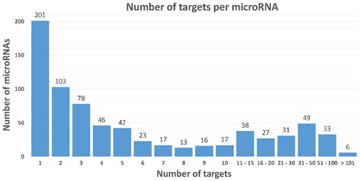
Distribution of the number of target genes per miRNA for humans in miRTarBase. The median number of targets is 3, upper quartile is 10 targets, and the maximum observed is 223 targets for one miRNA (miR-155-5p)

Unless these miRNAs are extremely abundant, their effect in vivo should be minor (Saçar Demirci et al., 2019).

2.2 maTE algorithm

The maTE algorithm considers miRNAs and their target gene expression for two conditions: control (negative) and disease (positive). Each condition is represented by their gene expression values for the experiment (each sample contributes one feature). The main motivation for the algorithm is that it is not known a priori which miRNAs may be involved in causing diseases. Therefore, machine learning is used to learn which miRNAs are associated with gene expression (Fig. 2), leveraging knowledge learned in previous studies (AbdAllah et al., 2017; Yousef et al., 2007, 2009). One of the main components of the maTE tool is the ranking stage R() (see Algorithm 1).

Fig. 2.

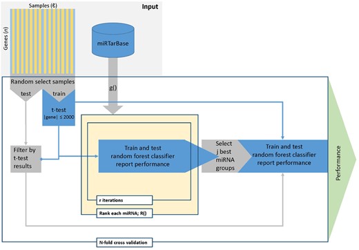
maTE work flow. The two main steps of the workflow are creating models for each miRNA (center) and then combining multiple miRNAs into one model and training a classifier using these miRNAs. Input: samples are horizontal with the two classes represented as lighter and darker stripes. Genes are represented by the vertical bars. miRTarBase depicts the miRNA target data from miRTarBase. Loops are represented by rectangles with a tag (e.g. N-fold cross-validation). The t-test calculations are based on the training data, but filtering is applied to the genes in both training and testing data

The expression of each gene (typically thousands) in the gene expression dataset represents a feature. Features are grouped by the miRNAs that can target them according to miRTarBase (the median is three targets per miRNA). For example, one group related to the hsa-let-7a-3p miRNA contains the target genes CCND1, CCND2 and E2F2, and another group related to hsa-let7d-5p contains the genes HMGA2, APP, DICER1, SLC11A2, IL13, MPL, AGO1, TNFRSF10B and COL3A1. miRNAs may share all or a subset of their targets. The gene DICER1 is targeted by 20 miRNAs, e.g. by miR-581 and miR-3928-3p. For the latter, it is the only currently known target while miR-581 also targets EDEM1. For another example, about 20 miRNAs target both PTEN and BCL2 among other targets.

Algorithm 1.

The Ranking method R(), a main component of the maTE algorithm.

Ranking Algorithm -  $\mathit{R}({\mathit{X}}_{\mathit{s}},\mathit{g}(\mathit{M}),\mathit{f},\mathit{r})$

  X_s: any subset of the input gene expression data X, the features are gene expression values

  M {${\mathit{m}}_1,{\mathit{m}}_2,\dots ,{\mathit{m}}_{\mathit{p}}\}$ is a list of miRNAs

  Grouping function g(M)- for each m_i, associate the names of genes (Genes ID) that are targeted by miRNA m_i(See Table 2).

  fis a scalar ($0\le f\le 1$⁠): split into train and test data

  r: repeated times (iteration)

  res={} for aggregation the scores for each m_i

Generate Rank for each m_i-Rank(m_i):

 For each m_i in M

  sm_i=0;

  Perform r time (here r = 5) Steps 1–5:

1. Perform stratified random sampling to split X_s into train X_t and test X_v datasets according to f (here 80:20)

2. Remove all genes (features) from X_t and X_v which are not targets of m_i

3. Train classifier on X_t (here Random Forest)

4. t = Test classifier on X_v—calculate performance

5. sm_i = sm_i + t;

 Score(m_i)= sm_i /r; Aggregate performance

 res= $\underset{i=1}{\overset{p}{\cup }}\mathit{Score}\left(m_i\right)$

Output

Return res (res = {Rank(m₁), Rank(m₂),…, Rank(m_p)})

In the following, we define the maTE algorithm, which consists of the miRNA-gene ranking (Algorithm 1) and the integration parts (Algorithm 2).

2.2.1 Ranking lists of genes associated with miRNAs

Let X denotes a two-class gene expression dataset consisting of ℓ covariate samples and n genes (Fig. 2, input). The classes could be disease and control, or any experimental condition versus a control or another experimental condition.

Let g() be a function grouping genes into clusters. Here, g() can be any algorithm which groups genes. For example, Yousef et al. (2007) previously used the k-means algorithm for grouping by gene expression. For the maTE algorithm, g() is provided by miRNAs and their targets. For example, g(hsa-let-7a-3p) groups the genes CCND1, CCND2 and E2F2 (see Table 2). More formally, let g(m_i) define the grouping based on the m_i miRNA’s targets (i: index of miRNAs available in miRTarBase). We chose to use miRTarBase, but other databases such as TarBase or computationally predicted targets would provide other/additional valid options. Note that the number of targets varies with the chosen miRNA (Fig. 1).

By iterating over all g(m_i), the miRNAs are ranked according to their ability to differentiate the two classes based on the test outcomes following training of a random forest (RF) classifier using an 80:20 split into training and testing data (Fig. 2: yellow section). First, the grouping function g(m_i) extracts the relevant gene expression data rows from X and then RF is applied. The ranking function is defined as R(X_s, g(m_i), f, r), where X_s is any subset of X, f defines the data split into training and testing (here, f is 80:20), r is the number of repetitions (here 5), and R() then returns the average accuracy. The pseudo code is provided as Algorithm 1.

Algorithm 2.

The overall algorithm of maTE, which depends on the R() method (see Algorithm 1).

maTE Algorithm

Objective

 maTE aims to select j miRNAs with target genes that can best classify samples by expressions.

Input

 X: gene expression data with two-class labels, the features are genes expression.

 M {${\mathit{m}}_1,{\mathit{m}}_2,\dots ,{\mathit{m}}_{\mathit{p}}\}$: list of miRNAs (here from miRTarBase) where p is the number of miRNAs.

 Grouping function g(M)- for each m_i associate the names of genes (Genes ID) that are targeted by miRNA m_i(See Table 2).

Algorithm

 M*={} empty list

 Perform N-fold cross-validation (here N = 100):

  Randomly split data by samples into train (X_t) and test (X_v) parts,

   performs Steps 1–6:

1. X_tf = filter genes (features) from training data by t-test (here P-value ≤ 0.05 and maximum number of filtered genes ≤ 2000)

2. X_vf = remove all genes from X_v that are not in X_tf

3. miR_p = R(X_tf, g(M), f, r) (here f = 80:20 with stratified random sampling; r = 5). R() is the procedure in Algorithm 1, the output will be miR_p ={Rank(m₁), Rank(m₂),…, Rank(m_p)}

4. M*= Sort( miR_p) according to performance; best first

5. M* = {m*₁, m*₂,.., m*_j}, Select best j miRNAs (here j = 2)

6. Filter X_tf and X_vf by g(M* ), now X_tf and X_vf represented by genes that are targeted by miRNA from M*.

 Train classifier using X_tf and X_vf (here random forest)

 Test classifier using X_vf

Output

 Report performance (e.g. average accuracy)

2.2.2 Integration

Following the ranking step for each miRNA as the grouping factor, the best j miRNAs (we set j to 2) are selected and their groups (i.e. their targets) are combined (Fig. 2, yellow section). An RF model is trained with the g() provided by the best j miRNAs instead of just m_i. The model is tested, and the performance measures are recorded.

We performed the complete procedure 100 times using MCCV (Fig. 2: N-fold Cross-validation loop). For each fold, the input is stratified random sampled and split into training and testing sets. The training set is submitted to t-test analysis. At maximum, 2000 differentially expressed genes with a P-value below 0.05 are selected. The selected genes are then used to filter the test dataset so both datasets contain the same genes. Within each iteration, the miRNAs are first ranked and then the best j miRNAs are used to train an RF classifier combining the j best miRNAs. The pseudo code is available as Algorithm 2.

2.2.3 Workflow

The algorithms we developed can be implemented in many systems. In order to test our approach and provide a proof of principle as well as an interface for users, we developed the approach using the Konstanz Information Miner (KNIME). The resulting KNIME workflow (Fig. 3) is available for download from Bioinformatics online and https://malikyousef.com/. The workflow in Figure 3 consists of processing nodes and data connections (lines/edges). Data travel along the edges through the workflow. For better readability and to increase modularity, meta-nodes (grey nodes, e.g. ‘Preprocess incl. t-test’) encapsulate sub-workflows. Workflow control includes programing constructs such as loops (blue nodes) and branching. The maTE workflow in Figure 3 contains user input in the orange boxes and presents the results in the green box. Processing is performed in the yellow and blue box. The green dots under the nodes indicate that the process has successfully succeeded.

Fig. 3.

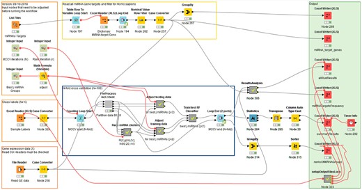
maTE work flow. Overview of the KNIME workflow available at Bioinformatics online. Input that needs to be adjusted is in the boxes to the left. The central box contains the MCCV and further logic is encapsulated in meta-nodes such as PreProcess and R(). Results are stored within the box on the right based on the location of the files with the class labels which can be adjusted in Node 323 (Y bottom of righthand box) if desired

2.3 Classification approach

We used the RF classifier implemented by the KNIME platform (Berthold et al., 2008). The classifier was trained and tested with a split of 80% training and 20% testing data. We have considered the under-sampling balancing approach to analyze imbalanced data. The under-sampling balancing approach is reducing the size of the abundant class by keeping all samples in the rare class and randomly selecting an equal number of samples in the abundant class. This approach is repeated during each round of cross-validation. We implement 100-fold MCCV (Xu and Liang, 2001) for model training. We used the default RF parameters where the split criterion is the information gain ratio. We did not limit the number of levels (tree depth), and the number of models was set to 100. Slight changes to these values did not change the overall performance.

2.3.1 Model performance evaluation

For each established model, we calculated a number of statistical measures such as sensitivity, specificity and accuracy to evaluate model performance. The following formulations were used to calculate the statistics (TP, true positive; FP, false positive; TN, true negative; and FN, false negative):

Sensitivity (SE, Recall) = TP/(TP + FN)

Specificity (SP) = TN/(TN + FP)

Accuracy (ACC) = (TP + TN)/(TP + TN + FP + FN)

All reported performance measures refer to the average of 100-fold MCCV. The positive class and negative class for each data are described in Table 1.

2.4 Recursive cluster elimination

We have previously developed a different method with a similar aim, SVM-RCE (Yousef et al., 2007), and later compared the methodology with other approaches (AbdAllah et al., 2017; Yousef et al., 2009). Although there are similarities in the general idea of using classification, the methods differ in the way genes are grouped. The SVM-RCE algorithm groups gene expression based on the k-means clustering algorithm’s grouping of the gene expression data (intrinsic information). Our novel approach (maTE) groups gene expression data based on information about miRNAs and their target genes (extrinsic information). The SVM-RCE algorithm performs three steps: (i) the clustering step groups the genes into clusters based on k-means; (ii) the scoring step evaluates the importance of each cluster of genes by internal cross-validation; and (iii) the RCE step removes the clusters with lower scores and is repeated until a desired number of clusters is obtained. In order to benchmark our novel approach, we performed a SVM-RCE analysis on all datasets used in this study using the default settings presented by (Yousef et al., 2007).

3 Results and discussion

We previously showed that for categorizing miRNAs into species, using machine learning, a minimum of 100 examples was needed (Yousef et al., 2017a, b). Therefore, we selected datasets with large numbers of samples (Table 1). In these datasets, patient and control samples are indicated, but miRNAs that lead to changes in mRNA expression and those that do not are unknown and unlabeled a priori. However, classification, in general, depends on annotated positive and negative data. Here, we use classification such that the annotation of which miRNA is significantly different between the two classes can be learned without the need for annotated examples. This objective can be accomplished by creating an abundance of machine learning models from the data. The model performance on the withheld test data indicates whether the model effectively separates classes, and a better performance more likely indicates a biological explanation. Here, our interest was to determine the miRNAs that best describe the differential mRNA expression between patient and control samples. However, the same approach could be used to answer many other biological questions such as pathway enrichment.

We applied both our novel methodology maTE and our previous related algorithm, SVM-RCE, to the selected data in Table 1 (Table 3). Our novel approach, maTE, searches for significant miRNAs and their targets, thereby limiting the search space to significantly differentially expressed ones, while SVM-RCE searches for significant genes in the complete space, not considering extrinsic grouping factors such as miRNAs. Table 3 summarizes the result of hundreds of thousands of trained models. The results show that SVM-RCE (avg. acc.: 0.94) outperforms maTE (avg. acc.: 0.78) for all datasets. However, SVM-RCE seems to be relatively indiscriminate and leads to all datasets having similar results because of the missing extrinsic grouping factor. Therefore, SVM-RCE or other approaches focusing on DE analysis might compile the effects of different regulatory mechanisms, whereas maTE focuses on effects caused by the miRNAs. maTE seems to discriminate between datasets where known miRNAs may not be the main cause of the observed difference in gene expression. Specifically, the differential gene expressions for datasets GDS2519, GDS3929 and GDS3646 do not seem to be caused by miRNAs, and the contributions of miRNAs seem to be low for the dataset GDS3268. Except for datasets GDS3646, GDS3929 and GDS2547, maTE generally collects more genes explaining the overall difference among states. The differences for the first two datasets are unlikely to be caused by miRNAs, and the difference in the results of the latter dataset may only have a limited contribution via miRNAs.

For the data analyzed, no ground truth is known; therefore, it is difficult to assign a confidence measure to our new approach. Some studies have measured mRNA and miRNA differential expressions (Enerly et al., 2011). It was our aim to use such data to benchmark our new method. Naively, the miRNAs selected by our algorithm should have high differential expressions between conditions. Unfortunately, this is not the case because many mRNAs are targeted by multiple miRNAs (Fig. 1), so a combined effect should also be considered. Our current approach is, however, miRNA centric and selects miRNAs that maximally explain the differential mRNA expression. The combined effects of miRNAs using our method are found by selecting the top j miRNAs (see Step 7 in the maTE algorithm). Here, we report results with j = 2. However, we have also tested different values of j such as 3, 4 and 5, and the results show that using these values of j lead to little improvement. In the future, we aim to optimize the set of miRNAs best able to separate the classes. The motivation for this optimization is the spikes in the trend in Figure 4. miRNAs with lower rank but high impact on the DE can cause such spikes. An optimization approach would be able to combine these miRNAs into a minimal set explaining a large part of the differential RNA expression.

Fig. 4.

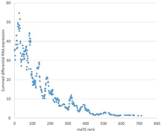
The maTE rank for miRNAs versus the sum of their absolute target differential expressions.

We applied maTE and SVM-RCE to a dataset of miRNA-mRNA breast tumors (Enerly et al., 2011) considering the mRNA expression of 15 basal-like and 41 luminal-A samples. These samples are the subtypes with the strongest reciprocal mRNA expression profiles (GO identifier GSE19536). We refer to this experiment as LumA_vs_Basal.

SVM-RCE ranks the importance of each gene by the number of times it appears on each RCE level. For example, if we start the process with the top 1000 genes selected by t-test from the training data and start with 100 clusters, then we have 27 levels of RCE (each time we reduce the number of clusters by 10%). We track the frequency of each gene in each level over 100 iterations. The score is the total number of frequencies divided by 2700 (100 iterations * 27 levels). The complete results for the top 1000 genes are available in Supplementary Material S2. The top gene is GATA3 that is required for the development of the mammary gland and has been implicated in breast cancer. MLPH (Rank 2) is also a marker for breast cancer survival. Other genes in the top 10 such as BCMP11 are also implicated in breast cancer. Thus, SVM-RCE collected relevant genes from the dataset. Because SVM-RCE does not assign any relevance to miRNAs, it cannot be compared with maTE on this dataset that consists of coordinated miRNA and mRNA measurements. Also, GATA3 was also part of three miRNA target sets in the top 10 miRNAs deduced by maTE. MLPH and BCMP11 were not found as targets because they were not available as targets in miRTarBase.

Some outcomes of the breast cancer study (Enerly et al., 2011) used here have also been confirmed in (Sandhu et al., 2014). Especially, miR-146a is overexpressed in basal-like breast cancer cells. However, some p53-dependent changes, including expression of miR-134, miR-146a and miR-181b, were found to be subtype specific. maTE also assigns some importance to miR-146a (Rank 30), but it is not within the top 10 of miRNAs explaining the difference between luminal and basal.

Because miRNAs can have several targets, we wanted to determine whether there is a correlation between the summed absolute differential expression of these targets versus the rank assigned by maTE. The expectation that more differential expression is explained in general with better ranks holds true (Fig. 4). This result shows that maTE fulfills the expectation and, at least for mir-146a, agrees with the previous results. Other miRNAs found to be important in separating luminal from basal type were mir-128, miR-17 (part of the miR-17–92 family) and the miR∼30 family (Iorio et al., 2005; see Enerly et al., 2011 and Sandhu et al., 2014). These miRNAs, or representatives of their families, are found in the top 20 of maTE assignments. As expected, some results differ among algorithms and the top assignments by maTE do not overlap with the findings by Enerly et al. (2011). For the top assignments, we submitted the deregulated targets to Reactome analysis and found that many of the miR-93 (Rank 1) targets are also under p53 control and involved in the PTEN pathway. Furthermore, the role of miR-93 (Rank 2) in breast cancer has previously been confirmed (Hao et al., 2018; Liang et al., 2017). The same is also true for miR-24 (Khodadadi-Jamayran et al., 2018; Yu et al., 2018). The targets of miR-24 (Rank 3) are involved in senescence control, and their downregulation will likely lead to the avoidance of cell death. Among the top 10, there is only miR-510 with a single target (SPDEF). Interestingly, SPDEF has been implicated with various cancer types such as breast cancer (Sood et al., 2017) and miR-510 (Guo et al., 2013). These findings confirm all top assignments of maTE to be implicated in breast cancer and thereby qualitatively validate the strategy employed.

In our experiments, we used 100 MCCV iterations, which can take a few hours on a regular personal computer. Therefore, we were interested in whether 100 iterations are necessary. Consequently, we recorded all miRNA ranks for the 100 iterations for the GDS3837 experiment. We then calculated the average rank for development per iteration i.e. the average of all ranks for each miRNA until the iteration. The development of the average rank is plotted for nine miRNAs (Fig. 5), including the highest ranked one (hsa-miR-876-3p) and the lowest ranked one (hsa-miR-935).

Fig. 5.

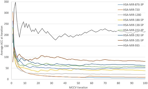
The development of the average rank for selected miRNAs for 100 MCCV iterations for the experiment GDS3837

Figure 5 shows that 100 MCCV iterations are not necessary. Additionally, we calculated how many iterations were needed for each miRNA to reach its average rank. The average number of iterations needed was about 24 iterations. Therefore, using fewer than 100 iterations seems adequate for future calculations.

4 Conclusion

The analysis of differential gene expression is employed in various biological scenarios such as differentiating between control and disease states. It has become clear that regulation occurs on many levels and that some regulatory switches cause a large downstream response while others lead to more subtle changes. miRNAs are both master switches and fine tuners of protein expression. One mode of the action of miRNAs leading to transcript degradation is accessible on the transcriptomic level.

One of the novelties of our approach, called maTE, is that we provide not just a significant list of deregulated genes, but also group them by their targeting miRNAs. To the best of our knowledge, this is the first account of such an approach. The generated information is very valuable to the biology community and will allow the addressing of novel biological questions.

We applied our approach to breast cancer data (Enerly et al., 2011) and were able to confirm some of the previous findings. However, the top assignments made via maTE indicate different miRNAs and corresponding targets than in the original assessment. Interestingly, the maTE assignments have clear associations with breast cancer, and this result is missing in the original study.

In the future, maTE can be extended with existing tools. For example, MetaMirClust (Chan et al., 2012) deduces miRNA clusters, and using a grouping function based on such clusters instead of single miRNAs would be worth considering for maTE, assuming the coordinated transcription of miRNA clusters. MAGIA² (Bisognin et al., 2012) and CSMirTar (Wu et al., 2017) can be employed as an alternative to miRTarBase to have a more comprehensive list of target genes per miRNA. MAGIA² and miRConnX (Huang et al., 2011) can further be utilized to construct regulatory circuits and perform pathway enrichment following the relevant detection of miRNAs by maTE. In order to filter maTE input, miSEA (Çorapçıoğlu and Oğul, 2015) can be employed to reduce the number of miRNAs for datasets where both miRNA and mRNA expression are available.

Although maTE selects the top j (here 2) miRNAs, in the future, it would be beneficial to determine a minimal network of miRNAs and their targets that maximizes the amount of differential expression among states. To achieve this objective, we aim to add an optimization step embedding the yellow part of the algorithm (Fig. 2) using, e.g. a genetic algorithm.

Funding

The work was supported by the Zefat Academic College to M.Y.

Conflict of Interest: none declared.