Enhanced Waddington landscape model with cell–cell communication can explain molecular mechanisms of self-organization

Abstract

Motivation

The molecular mechanisms of self-organization that orchestrate embryonic cells to create astonishing patterns have been among major questions of developmental biology. It is recently shown that embryonic stem cells (ESCs), when cultured in particular micropatterns, can self-organize and mimic the early steps of pre-implantation embryogenesis. A systems-biology model to address this observation from a dynamical systems perspective is essential and can enhance understanding of the phenomenon.

Results

Here, we propose a multicellular mathematical model for pattern formation during in vitro gastrulation of human ESCs. This model enhances the basic principles of Waddington epigenetic landscape with cell–cell communication, in order to enable pattern and tissue formation. We have shown the sufficiency of a simple mechanism by using a minimal number of parameters in the model, in order to address a variety of experimental observations such as the formation of three germ layers and trophectoderm, responses to altered culture conditions and micropattern diameters and unexpected spotted forms of the germ layers under certain conditions. Moreover, we have tested different boundary conditions as well as various shapes, observing that the pattern is initiated from the boundary and gradually spreads towards the center. This model provides a basis for in-silico modeling of self-organization.

Availability and implementation

https://github.com/HFooladi/Self_Organization.

Supplementary information

Supplementary data are available at Bioinformatics online.

1 Introduction

From a long time ago, a great number of prominent scientists devoted their lives to think about how biological patterns emerge and how differentiation occurs (e.g. Gierer and Meinhardt, 1972; Turing, 1952; Wolpert, 1969). Different cell fates that organize through space and time are formed from seemingly identical ones. In 1957, Waddington depicted a well-known epigenetic landscape, which unveils how a cell commits to different cell types starting from an undifferentiated state (Waddington, 1957). This model has been inspiring for more than a decade and triggered a significant number of works on cell fate decision making and envisioning cell fates as high-dimensional attractor states of a complex gene regulatory network (Huang et al., 2005; Mojtahedi et al., 2016). Despite a highly profound and influential vision, it does not provide sufficient clues on how diverse patterns emerge in the coordination of cellular population. The missing component of this model is cellular communication.

Cells communicate with each other in different ways, and communication plays a central role in their development. Mechanical and chemical signaling (e.g. autocrine, endocrine, paracrine and direct cell–cell contact) are considered as the two major modes of cellular interaction (Howard et al., 2011). For instance, reaction-diffusion models are considered as paracrine signaling, while delta-notch signaling is within the category of direct cell–cell contact (Phillips et al., 2012).

Lewis Wolpert proposed one of the earliest models for explaining pattern formation, known as positional information (PI) model, in 1969 (Wolpert, 1969). This model suggests a specific embryonic region diffuses some chemical substance, so-called morphogen, which results in a morphogen gradient formation. Cell fate is the function of a morphogen concentration that a cell receives (Wolpert, 1969). Positional information model does not account morphogen interactions and consequently is incapable of producing oscillatory patterns (Kondo and Miura, 2010). From another point of view, Alan Turing proposed the reaction-diffusion (RD) model, which is based on the interaction of two morphogens and can produce oscillatory patterns (Turing, 1952). The RD model can explain the formation of different biological patterns such as animal skin patterns, and vasculogenesis (Gierer, 1981; Kondo and Miura, 2010; Koch and Meinhardt, 1994; Maini et al., 2012). Furthermore, it is possible to combine RD and PI and create another sophisticated biological model (Green and Sharpe, 2015).

There are numerous examples of pattern formation during early human embryo development, and gastrulation is among the most important of them. Lewis Wolpert has stated, ‘it is not birth, marriage, or death, but gastrulation which is the most important time in your life’ (Vicente, 2015) unveiling the significant importance of gastrulation. Gastrulation is a self-organized process; which means without any external force, and only by cell–cell communication, a group of identical cells differentiates and forms an ordered spatial pattern. During mammalian gastrulation, epiblast cells in blastocoel were differentiated from inner cell mass, produced three main kinds of cells: ectoderm, mesoderm and endoderm. These three spatially organized layers are the progenitor of almost every cell in the human body (Deglincerti et al., 2016a,b).

It has been shown recently, that providing geometric confinement is enough for recapitulation of the sequentially ordered pattern. This finding opened new doors for studying this process more precisely in great depth (Deglincerti et al., 2016a,b; Warmflash et al., 2014). In this experiment, homogenous BMP4 was used as an input signal for triggering self-organized gastrulation, and cells were confined to circular microcolonies of 250 to 1000 μm diameter. They investigated the effect of micropattern sizes and different concentrations of initial BMP4 on output pattern experimentally (Warmflash et al., 2014). Etoc et al. (2016) followed this procedure and proposed a mathematical model, explaining this qualitative behavior (Etoc et al., 2016). As a result, they found out initial receptor relocalization and interaction of BMP4 and its inhibitor, Noggin, were responsible for ordered germ layer formation. Although their suggested mathematical model was compatible with the previous experiment, it was not rich enough to produce an oscillatory pattern observed in later experiments (Tewary et al., 2017). Tewary et al., (2017) showed that by increasing colony diameter and initial BMP4 concentration, the spotty pattern arises (Tewary et al., 2017). They modified (Etoc et al., 2016) genetic circuit and added auto-regulation link for BMP4 which makes this model capable of producing spatial oscillation, and their proposed model resembles the Turing model in mind.

In spite of being in agreement with the previous experimental results, providing a biologically plausible interpretation of model parameters is not straightforward. Correspondence between parameters and specific biological or molecular property is not clear. This restricts biologists from designing new experiments to verify the applicability of this model. i.e. it is not clear how the variation of parameters map to concrete biological factors (e.g. the production rate of BMP4) through in vitro experiments. Furthermore, another thing that makes this model inconvenient from our perspective is ignorance of cell identity. The previous model (Tewary et al., 2017) assumes the homogenous distribution of BMP4 and Noggin as a continuous field, and from their interaction, the sequential ordered pattern arises. However, a more precise and realistic model (i.e. model that remains mathematically rigorous, and at the same time, provide biologically testable predictions) should include cells as the core element and incorporate cell–cell communication.

We propose a mathematical model based on the dynamical system theory for justifying pattern formation during in vitro hESC gastrulation. This model not only is compatible with all the previous experiments but also considers cells as the main elements and contains parameters which have accurate and concrete biological interpretation. Moreover, it provides an opportunity for making testable biological statements about how the pattern varies in response to perturbing parameters.

Our model is generic and capable of supporting different forms of communication (such as direct contact) by slight modification in its implementation. This flexibility comes from considering cells as separate entities and secreting molecules in the extracellular space. In the proposed model, we have assumed diffusion as the mechanism of cellular interaction. To the best of our knowledge, this assumption is consistent with the existing literature about BMP4-Noggin interaction (Etoc et al., 2016; Warmflash et al., 2014).

2 Materials and methods

We proposed a model based on the dynamical systems approach. The minimal genetic circuit has been considered inside each cell, and this circuit contains the interaction of BMP4 and Noggin genes which are among the essential genes in human gastrulation. In particular, BMP4 activates production of Noggin and itself, and Noggin inhibits production of BMP4 (Fig. 1a). It is biologically well-known that BMP4 does not interact with Noggin directly; it first stimulates phosphorylation of Smad1 and complex of Smad1 and Smad4 transfer to the nucleus and activates Noggin expression (Gromova et al., 2007). But, in the proposed model, we have ignored these intermediate steps for the sake of simplicity. This circuit can be considered as a dynamical system and the underlying equations that capture these interactions can be derived. Each gene has a degradation rate as well as production rate.

$$\frac{d}{\mathit{dt}}N=\frac{{\beta }_N{\left(\frac{B}{K_{\mathit{BN}}}\right)}^n}{1+{\left(\frac{B}{K_{\mathit{BN}}}\right)}^n}+a_N-{\alpha }_{N}N\hspace{1em} B:\mathit{BMP}4,N:\mathit{Noggin}$$

(1)

$$\frac{d}{\mathit{dt}}B=\frac{{\beta }_B{\left(\frac{B}{K_{\mathit{BB}}}\right)}^n}{1+{\left(\frac{B}{K_{\mathit{BB}}}\right)}^n+{\left(\frac{N}{K_{\mathit{NB}}}\right)}^n+{\left(\frac{B.N}{K_1}\right)}^n}+a_B-{\alpha }_{B}B$$

(2)

Fig. 1.

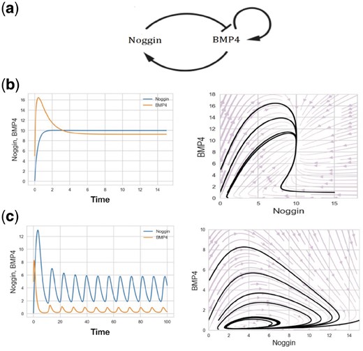
(a) Genetic circuit that shows interaction of BMP4 and Noggin genes. (b) Behavior of the genetic circuit in time and state space. Evolution of the system when the parameters have been selected based on the first row of Table 1. (c) Evolution of the system when the parameters have been selected based on the second row of Table 1. Left: Time-space. Right: State space, starting from different initial conditions

Table 1.

Two sets of parameters that can cause two completely different qualitative behaviors

${\tilde{a}}_N$	${\tilde{a}}_B$	${\tilde{\beta }}_B$	${\tilde{\beta }}_N$	λ	r  1	r  2	n
0.1	1	100	10	3	0.1	1	2
0.1	0.1	20	20	0.4	0.1	1	2

In this equation, N is the concentration of Noggin and B is the concentration of BMP4 in one cell. α_B and α_N stand for degradation rates of BMP4 and Noggin in each cell respectively. Furthermore, β and a are the production rates, and K represents the binding affinity of one protein to the dedicated promoter.

Since this equation plays a significant role in the subsequent analysis, it is essential to clarify the logic behind its derivation. Moreover, a detailed interpretation of each variable in the equation can be elucidating. So, consider the first equation which capture the variation of Noggin over time:

• Change of one protein concentration over time has been written as a combination of production and degradation of this protein (Huang et al., 2007). As a result, first and second terms in the Equation 1 correspond to the production of Noggin, and the third term refers to the degradation of Noggin in a cell.

• The first term is the feedback-dependent component of Noggin synthesis. BMP4 acts as an activator of Noggin synthesis and this term captures this effect. It is important to note that often biological response function is approximated as Hill-function (Ferrell, 2012). β_N represents the maximum rate of feedback-dependent production of Noggin. Another parameter K_BN is called activation coefficient and corresponds to the concentration of BMP4, which is necessary to significantly activate the production and synthesis of Noggin. The unit of this parameter is concentration, and it depends on the chemical binding affinity of BMP4 to the Noggin promoter (Alon, 2006). Since the BMP4 does not directly activate Noggin and this activation is done within the cascade of events and intermediation of other proteins, K_BN only models the effect of binding affinity. The last parameter of this term is n, which determines the steepness of the Hill-function; the higher n corresponds to a steeper hill-function, and leads to a more switch-like behavior. Often in the biological systems, n is considered to be in the range of 1–4 (Alon, 2006).

• The second term is called the basal rate of Noggin synthesis and corresponds to the rate of Noggin synthesis in the absence of BMP4 and other activators (Ferrell, 2012). Even in the absence of an activator, an RNA polymerase can bind to Noggin Promoter and synthesize Noggin in this situation. Consequently, a_N is the basal production rate and can be experimentally determined by measuring the rate of Noggin Synthesis in the absence of BMP, e.g. by knocking down the BMP4 and measuring the concentration change of Noggin.

• The last term refers to the degradation and dilution of Noggin within a cell (Alon, 2006). The concentration of the protein decreases within the cell because of two reasons. First, the expansion of a cell and consequently, dilution of the protein and the second reason is the active degradation of the protein by an enzyme called protease. There is a correspondence between α and the half-life of the cell (Alon, 2006), which makes it easy to measure and determine α.

Now consider Equation 2 which belongs to the variation of BMP4 within a cell. The logic behind the derivation of this equation is very similar to Equation 1, but there are subtle differences that require clarification. Like Equation 1, this one again contains production of BMP4 as well as degradation. The first and second term relates to production, and the last term represents the degradation of BMP4 within a cell. The second term is the basal expression of BMP4, and the third term relates to dilution and degradation of BMP4. Only the first term is a little ambiguous and needs more details for elucidation. The first term is the feedback-dependent component of BMP4 synthesis. Two processes contribute to this synthesis: the first one is auto-activation of BMP4, and the second one is cross-inhibition of BMP4 by Noggin. Again, this synthesis can be written in the form of hill function which originates from intracellular physiochemical conditions (Huang et al., 2007). Since there are two regulators, one activator and one repressor, there exists two interacting promoter sites for regulation of BMP4. The first term can be re-written as the following:

$$\frac{{\beta }_B{\left(\frac{B}{K_{\mathit{BB}}}\right)}^n}{1+{\left(\frac{B}{K_{\mathit{BB}}}\right)}^n+{\left(\frac{N}{K_{\mathit{NB}}}\right)}^n+{\left(\frac{N.B}{K_1}\right)}^n}={\beta }_B.F_{\mathit{reg}}$$

(3)

In the case of two interacting regulatory sites, F_reg can be written as the following (Bintu et al., 2005; Goentoro et al., 2009):

$$\frac{{\left(\frac{B}{K_{\mathit{BB}}}\right)}^n}{1+{\left(\frac{B}{K_{\mathit{BB}}}\right)}^n+{\left(\frac{N}{K_{\mathit{NB}}}\right)}^n+{\left(\frac{N.B}{K_1}\right)}^n}=F_{\mathit{reg}}$$

(4)

In one specific case, when there is no interaction between BMP4 and Noggin promoter sites, the situation becomes simpler and can be written as the product of two regulatory terms:

$$\begin{array}{c}{F}_{\mathit{reg}}=F_{\mathit{reg}1}.F_{\mathit{reg}2}=\frac{{\left(\frac{B}{K_{\mathit{BB}}}\right)}^n}{1+{\left(\frac{B}{K_{\mathit{BB}}}\right)}^n}.\frac{1}{1+{\left(\frac{N}{K_{\mathit{NB}}}\right)}^n}\hfill \\ =\frac{{\left(\frac{B}{K_{\mathit{BB}}}\right)}^n}{1+{\left(\frac{B}{K_{\mathit{BB}}}\right)}^n+{\left(\frac{N}{K_{\mathit{NB}}}\right)}^n+{\left(\frac{N.B}{K_{\mathit{BB}}.K_{\mathit{NB}}}\right)}^n}=F_{\mathit{reg}}\hfill \end{array}$$

(5)

In the proposed model, a more general case, i.e. two interacting regulatory sites, has been considered. In Equation 5, K_BB and K_NB represent the binding affinity of BMP4 and Noggin to BMP4 promoters respectively. There is a probability of binding of BMP4 to the BMP4 promoter and K_BB reflects the effect of this probability. Although there is no direct link between Noggin and BMP4, and Noggin influences the production of BMP4 through the downstream pathway indirectly, for the sake of simplicity, we have summarized all these interactions in the parameter K_NB.

Moreover, it is worth noting that all the parameters in the equations can be easily measured and determined in practice by means of experimental observation. The only parameters that are not very convenient for measurement are binding affinities (K), since lots of interaction has been summarized and abstracted in these parameters.

2.1 Dimensionless equations

It is a reasonable idea to use non-dimensional version of dynamical system equations. Nondimensionalization often reduces the number of free parameters, and consequently reduces search space. It is important to choose appropriate dimensionless parameters. We chose dimensionless parameters as shown in the following equations:

$$\begin{array}{c}\tilde{t}={\alpha }_{B}t\tilde{N}=\frac{N}{K_{NB}}\tilde{B}=\frac{B}{K_{BB}}\widetilde{{\beta }_N}=\frac{{\beta }_N}{{\alpha }_N.K_{NB}}\\ \widetilde{{\beta }_B}=\frac{{\beta }_B}{{\alpha }_B.K_{BB}}\lambda =\frac{{\alpha }_N}{{\alpha }_B}\widetilde{a_N}=\frac{a_N}{{\alpha }_N.K_{NB}}\widetilde{a_B}=\frac{a_B}{{\alpha }_B.K_{BB}}\\ r_1={\left(\frac{K_{BB}.K_{NB}}{K_1}\right)}^n{r}_2={\left(\frac{K_{BB}}{K_{BN}}\right)}^n\end{array}$$

(6)

Manipulating the original equations with dimensionless parameters can lead to the following results.

$$\begin{array}{c}{\lambda }^{-1}\frac{d}{d\tilde{t}}\tilde{N}=\widetilde{{\beta }_N}\frac{r_2{\tilde{B}}^{\mathit{n}}}{1+r_2{\tilde{B}}^{\mathit{n}}}+\widetilde{a_N}-\tilde{N}\hfill \\ \frac{d}{d\tilde{t}}\tilde{B}=\widetilde{{\beta }_B}\frac{{\tilde{B}}^{\mathit{n}}}{1+{\tilde{B}}^{\mathit{n}}+{\tilde{N}}^{\mathit{n}}+r_1{\tilde{A}}^{\mathit{n}}{\tilde{B}}^{\mathit{n}}}+\widetilde{a_B}-\tilde{B}\hfill \end{array}$$

(7)

Detailed description of the derivation of Equation 7 can be found in the Supplementary Material (Appendix A). Equation 7 consists of eight free parameters, searching through which, can lead to different qualitative behaviors. We simulated and tested about 100 different sets of parameters. Observed qualitative behaviors can be classified into two dominant regimes: approaching the fixed points and oscillatory behavior. When it is approaching the fixed points, the steady state concentration of Noggin can be either higher, or lower than that of BMP4. Furthermore, we observed various transient behaviors during convergence to the fixed points in terms of monotonicity. In the second case, oscillation with different frequencies and amplitudes for Noggin and BMP4 have occurred during simulations. Figure 1b and c and Table 1 represent a sample simulation and associated parameters for each mentioned behaviors.

2.2 Incorporating cell–cell communication via diffusion

In Section 2.1, we only consider one particular cell and derive the corresponding equation for that. However, when dealing with cellular population, interaction plays an important role and must be somehow reflected in the model (Fig. 2a). Without considering interaction, the connection of the model with reality becomes obscure and the model would deviates from reality. Although there are different ways for cellular communication, in this paper cell–cell interaction occurs via diffusion. Our goal in this paper is to consider the population of cells, placing the genetic circuit in each cell, and provide communication through diffusion. BMP4 and Noggin proteins can leave the surface of the cells, diffuse through extracellular space, penetrate through the surface of the other cells, and subsequently influence the behavior of other cells in the environment (Equations 8 and 9). In this manner, we have incorporated cellular interaction in our model which is one of the key parts in pattern formation (Kondo and Miura, 2010).

$$\frac{d}{\mathit{dt}}N=\frac{{\beta }_N{\left(\frac{B}{K_{\mathit{BN}}}\right)}^n}{1+{\left(\frac{B}{K_{\mathit{BN}}}\right)}^n}+a_N-{\alpha }_{N}N+D_N(\frac{{\partial }^{2}N}{\partial x^2}+\frac{{\partial }^{2}N}{\partial y^2})$$

(8)

$$\begin{array}{cc}\frac{d}{\mathit{dt}}B=\hfill & \frac{{\beta }_B{\left(\frac{B}{K_{\mathit{BB}}}\right)}^n}{1+{\left(\frac{B}{K_{\mathit{BB}}}\right)}^n+{\left(\frac{N}{K_{\mathit{NB}}}\right)}^n+{\left(\frac{B.N}{K_1}\right)}^n}+a_B-{\alpha }_{B}B\hfill \\ \hfill & +D_B(\frac{{\partial }^{2}B}{\partial x^2}+\frac{{\partial }^{2}B}{\partial y^2})\hfill \end{array}$$

(9)

Fig. 2.

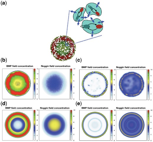
(a) Schematic of proposed model. (b–e) Comparison of pattern formation resulted from proposed model (top) with reaction-diffusion model (bottom). (b, d) Same qualitative but different quantitative behavior on 500μ colony. (c, e) Ring-shape pattern emerges from reaction-diffusion model, while spotty pattern appears from our model on 3000μ colony

Again, by choosing appropriate parameters, equations can become dimensionless and dealing with dimensionless equation is more convenient. The details of this derivation can be found in the Supplementary Material (Appendix B).

$${\lambda }^{-1}\frac{d}{d\tilde{t}}\tilde{N}=\widetilde{{\beta }_N}\frac{r_2{\tilde{B}}^n}{1+r_2{\tilde{B}}^n}+\widetilde{a_N}-\tilde{N}+{\tilde{D}}_N(\frac{{\partial }^2\tilde{N}}{\partial x^2}+\frac{{\partial }^2\tilde{N}}{\partial y^2})$$

(10)

$$\begin{array}{cc}\frac{d}{d\tilde{t}}\tilde{B}=\hfill & \widetilde{{\beta }_B}\frac{{\tilde{B}}^n}{1+{\tilde{B}}^n+{\tilde{N}}^n+r_1{\tilde{N}}^n{\tilde{B}}^n}+\widetilde{a_B}-\tilde{B}\hfill \\ \hfill & +{\tilde{D}}_B(\frac{{\partial }^2\tilde{B}}{\partial x^2}+\frac{{\partial }^2\tilde{B}}{\partial y^2})\hfill \end{array}$$

(11)

One of the key aspects of the proposed model is this fact that the BMP4 and Noggin can only be produced within the cells, and in extracellular space, the protein synthesis is zero. i.e. in the extracellular space, only degradation and diffusion can take place. The following are other assumptions:

1. Diffusion coefficient is constant throughout the space for both BMP4 and Noggin, which means diffusion is homogenous. It means that diffusion is not a function of space and is independent of the coordinate, which is not an odd assumption. It is not hard to make diffusion a function of space; but our goal is to keep the model as simple as possible while, capturing and conforming all the previous experiments and observations.

2. Diffusion is isotropic, which means that the diffusion constant is not a function of direction and remains the same in all direction. In real scenario and in-vivo experiment, diffusion varies in different directions due to different factors (Manno et al., 2017). We have ignored this fact for the sake of the simplicity of our model. It is possible to add this feature and make the model more complicated in future works. It is required to know the exact position of the cell nucleus and cell compartments such as cytoskeleton and microtubules in order to model anisotropic diffusion precisely (Trimble and Grinstein, 2015).

3. The degradation rate of proteins (α) inside and outside of the cells are different. Within the cell, active protein degradation is performed by an enzyme which is called protease (Schrader et al., 2009); as a result of this active degradation, the degradation rate is higher within the cell with respect to the outside of the cell. This difference in degradation rate has been considered in the proposed model.

Equations 10 and 11 contain some free parameters. We have selected the parameters according to Table 2. The logic behind this decision and sensitivity of the pattern formation w.r.t. parameters will be discussed more precisely in Section 3.4.

Table 2.

Appropriate parameters for the emergence of the desired pattern

${\tilde{a}}_N$	${\tilde{a}}_B$	${\tilde{\beta }}_B$	${\tilde{\beta }}_N$	λ	r  1	r  2	n	${\tilde{D}}_B=\frac{D_B}{{\alpha }_B}$	${\tilde{D}}_N=\frac{D_N}{{\alpha }_N}$
0.1	0.1	20	20	0.4	0.1	1	2	250	12 500

All simulations in the multicellular system have been done with Morpheus. Morpheus is an user-friendly software designed for simulating and studying multicellular systems (Starruß et al., 2014). Detailed description of implementation in Morpheus can be found in Appendix C in Supplementary Material.

3 Results and discussion

3.1 Communication model explains in vitro self-organization

We tested communication-less model, i.e. the model without considering cellular interaction (Fig. 1). While it provides a baseline for modeling some observations such as attractor (stable-steady) states or oscillation, it fails to model enigmatic features of the living organisms such as embryonic development and self-organization. We aimed to enhance the model in order to resemble the experimental observations of in vitro gastrulation, as performed by Warmflash et al. (2014). For that purpose, we developed a multi-cellular model in which the fate of each cell is determined by a genetic circuit that reconciles intrinsic interactions with extrinsic signals of cell–cell communication (see methods for more details).

According to the previous experiments, we expect BMP4 to decrease from the edge towards the center of the colony, while Noggin exhibits the opposite behavior in 500 μm colony (Etoc et al., 2016; Warmflash et al., 2014), which is exactly the same behavior we observed (Fig. 2b). After formation of the BMP4-Noggin pattern, the appearance of different cell fates and ordered germ layers can be explained based on positional information mechanism. Distribution of BMP4 and Noggin influence the production of SOX2, SOX17 and CDX2, which induce different cell fates during gastrulation. e.g. the region with the high concentration of BMP4 and low concentration of BMP4 (the center of the colony) produces more SOX2 which induces ectodermal fate.

Tewary et al. (2017) showed that by increasing colony diameter (3000 μm colony), the spotty pattern arises. We observed the similar behavior (Fig. 2c). This spotty pattern can disrupt the formation of germ layers in the gastrulation.

During simulations, we realized that diffusion of BMP4 and Noggin has a significant effect on the pattern. In agreement with the expectation, it has been observed that desired pattern emerges when diffusion of Noggin is significantly greater than BMP4 (Gierer and Meinhardt, 1972; Turing, 1952).

Moreover, it is worth noting to mention that parameters vary within a reasonable biological range (Table 2). The typical diffusion coefficient of protein within the cell is set around 10 μm² s⁻¹ (Alon, 2006). In addition, Tewary et al., (2017) considered diffusion rate of Noggin and BMP4 as the following:

$$D_B=10\hspace{0.17em}{\mu \mathrm{m}}^2{\mathrm{s}}^{-1}\hspace{1em}\hspace{1em}{D}_N=50\hspace{0.17em}{\mu \mathrm{m}}^2{\mathrm{s}}^{-1}$$

(12)

The typical degradation rate of proteins within the cell depends on the cell generation time, varying in the range of $0.01(\mathrm{s})-0.001(\mathrm{s})$

(Alon, 2006) and we have considered the same ranges for degradation rate of BMP4 and Noggin in proposed model.

$$\begin{array}{c}{\alpha }_B=0.01\hspace{1em}\hspace{1em}{\alpha }_N=0.004\hspace{1em}\hspace{1em}{D}_B=10\hspace{0.17em}{\mu \mathrm{m}}^2{\mathrm{s}}^{-1}\hspace{1em}\hspace{1em}{D}_N=50\hspace{0.17em}{\mu \mathrm{m}}^2{\mathrm{s}}^{-1}\\ \lambda =\frac{{\alpha }_N}{{\alpha }_B}=0.4\hspace{1em}\hspace{1em}{\tilde{D}}_B=\frac{D_B}{{\alpha }_B}=250\hspace{0.17em}{\mu \mathrm{m}}^2{\mathrm{s}}^{-1}\\ {\tilde{D}}_N=\frac{D_N}{{\alpha }_N}=12500\hspace{0.17em}{\mu \mathrm{m}}^2{\mathrm{s}}^{-1}\end{array}$$

(13)

3.2 Communication model has critical advantages over continuous reaction-diffusion models

Although our model resembles reaction-diffusion, there is one major difference that distinguishes our model. In the normal reaction-diffusion model, production and degradation of morphogenes take place in all points throughout the space; however, in the proposed model morphogenes are produced within the cells, and the rate of degradation is higher inside the cells (as a result of active degradation) in comparison with extracellular space. This major difference in modeling assumptions has led to different results in simulations (Fig. 2b–e). For example according to our model, as the colony size increases (Fig. 2c and e), a spotty pattern emerges; while in the case of the continuous reaction-diffusion model, ring-shape oscillation appears. Therefore, for a large colony size a different qualitative behavior emerged. For a normal colony size (500 μm), although the pattern looks similar in a qualitative manner (Fig. 2b and d), quantitative behaviors differ substantially. In our model, the ratio of BMP4 concentration at the edge with respect to its concentration at the colony center is in agreement with previous experiments [e.g. Fig. 6a and b of Etoc et al. (2016)]. But in the continuous model, BMP4 concentration is zero at the center.

As a result, considering cells as the separate entities and providing communication via diffusion, has made a significant change in pattern formation with respect to continuous RD models.

3.3 Boundary analysis determines necessity of inhibitor diffusion from the colony

Warmflash et al. (2014) suggested that diffusible inhibitors have an essential role in establishing the pattern. In order to prove this assumption, they blocked this diffusion by growing colony at the bottom of PDMS microcell. This alteration made the boundary fate formation fails, and by this experiment, they claimed that diffusing inhibitors out of colony boundary are pivotal factors for pattern formation. In order to examine our model, two available boundary conditions have been tested: constant and no-flux. No-flux condition is the same as putting the colony at the bottom of microcell, and constant boundary condition corresponds to regular growing. Figure 3 depicts the results after running the model for two types of boundary condition. No-flux boundary condition leads to vanishing fate determination. It demonstrates the compatibility of our model with previous experiments. Therefore, we used the ‘constant’ boundary condition throughout simulations.

Fig. 3.

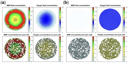
Simulation of proposed model in population of cells when the interaction and diffusion is present. These patterns have emerged after the transition time is over and when the system has reached the stable situation. (a) Simulation on 500 μm colony with constant boundary condition. (b) Simulation with no-flux boundary condition. Above: BMP4 and Noggin field in the environment. Below: Amount of BMP4 and Noggin within each cell

3.4 Local and global sensitivity analysis highlights parameters that influence in-silico self-organization outcome

One key advantage of the proposed model is providing a biological interpretation for each parameter. i.e. each parameter corresponds to the specific biological process or molecular properties. For example λ is the ratio of degradation of Noggin and BMP4 and varying λ means varying degradation rate of one of these proteins.

To get more insight into the model and its parameters, we have done sensitivity analysis. Sensitivity analysis (SA) is an important step in developing a biologically plausible mathematical model. SA methods can be divided into two general groups: local and global SA. Local SA approaches provide information about sensitivity of the pattern w.r.t each parameter when it deviates locally around a base point (by calculating derivatives or using more qualitative methods that are called ‘screening methods’). The main drawback of local methods is that derivatives provide information only around the base point where they are computed and do not take into account the rest of the variation range of the model parameters. Consequently, in order to explore all reasonable parameter ranges, global SA methods are introduced. Global approaches such as Morris methods (Campolongo et al., 2007; Morris, 1991) and variance-based methods (McKay et al., 1999; Sobol, 1993) efficiently sample from parameter space to analyze global importance and sensitivity of each parameter. Both global and local SA are performed for our parameters.

3.4.1 Local sensitivity analysis

For doing local SA, we have set the parameters according to Table 2 and we will call this set of parameters as base values. After that, each parameter varies in the vicinity of its base value and how the pattern changes are determined and measured (Fig. 4).

Fig. 4.

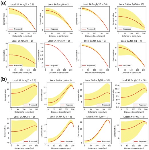
Local sensitivity analysis for each parameter in models for (a) Noggin, (b) BMP4 field in the circular colony

In Figure 4, y-axis corresponds to the concentration of Noggin (Fig. 4a) and BMP4 (Fig. 4b), and it can be observed how concentration changes along the radius of the colony. Red curve corresponds to the variation of concentration alongside the radius when the parameters have been set to the base values. Yellow region corresponds to the 95% interval of concentration in one specific radius. In order to plot this curve, first one specific radius is considered, then it is possible to measure how concentration changes in this specific radius in response to variation of one specific parameter. Mean and standard deviation of concentration for all the distances from the colony center has been calculated and 95% interval has been plotted. In addition, variation of pattern with respect to changes in diffusion has been examined and the result can be found in the Supplementary Material Appendix D. We observed that diffusion coefficients also have great impact on pattern formation.

Figure 4 reveals that the pattern is very sensitive to λ and β_N, and incremental change of these parameters can have a dramatic influence on the pattern. λ represents the ratio of degradation rates, and we can speculate that by interrupting degradation rate of Noggin or BMP4 (e.g. by blocking or interrupting active mechanism of degradation) we can disrupt the formation of germ layers.

3.4.2 Global sensitivity analysis

Morris methods are one of the most effective and robust methods in screening sensitivity analysis (Campolongo et al., 2007; Morris, 1991). The Morris method uses the mean (μ) and standard deviation (σ) of the some ‘elementary effects’ (local sensitivity features), measured at some special trajectories in order to provide an approximation of global importance of each parameter. This method has two outputs for each parameter: average and variance. The more the average is, the more important the parameter is. Higher standard deviation implies the non-linearity effect of the parameter or the result of interactions with other inputs. One of the drawbacks of Morris method is where there are some negative elements among our model output and they cancel out each other in mean operation and consequently reduce the reliability of the average feature as a measure for the importance of the parameter (Campolongo and Saltelli, 1997). In these situations, scientific advice is to use mean absolute value (⁠${\mu }^{*}$⁠) instead of the mean value to overcome this drawback (Saltelli et al., 2004).

We applied the Morris method for analyzing sensitivity and importance of parameters of the proposed model. The result has been shown in Figure 5. According to the result, importance of β_N, β_B, λ and r₁ is obvious in comparison with r₂, a₁ and a₂. High sensitivity to β_N and β_B was predictable because they are directly related to the production of Noggin and BMP4 respectively (i.e. blocking production by knocking down BMP4 or Noggin gene, obviously alters the patterns). But the high ${\mu }^{*}$ value for λ and r₁ implies the importance of the ratio of degradation rates and corporative bounding coefficient as well in pattern formation. So, variation of these parameters can significantly change the final pattern and accordingly germ layer fates.

Fig. 5.

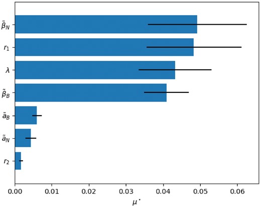
Morris method sensitivity analysis result. Parameters are ranked with respect to their ${\mu }^{*}$ as a measure for importance and high sensitivity

3.5 Predicting the effect of colony geometry on self-organization

In this section, we investigate the effect of geometry on the final pattern. Simulations were performed in two categories: circular and non-circular boundary confinement. All in vitro experiments have been done in a circular environment, but in natural gastrulation, a more complex situation is happening. So we decided to take this step further by simulating our model for more diverse and real geometries.

3.5.1 Circular geometry

Tewary et al., (2017) reported that by increasing colony diameter to around 3 mm, the spotty pattern will appear. In fact, our model leads to the same observation and we can see the desired pattern after simulation (Fig. 6a). For spotty pattern, we noticed that spots appear and oscillate through time until the system reaches a stable point and oscillation in time vanishes. Sensitivity analysis is also performed in order to investigate how much pattern varies in response to variation of the radius of the colony (Fig. 6b). The process is the same as what has been mentioned in Section 3.4.1. According to the result, a small alteration in colony radius can cause significant variation in BMP4 (Noggin) concentration and subsequently can change cellular fate determination; especially in cells closer to the center are more under the influence of variation of colony diameter (ectodermal and mesodermal fates). Warmflash et al., (2014) observed the vanishing of central fates when they reduced colony size, perfectly matching to our sensitivity analysis result.

Fig. 6.

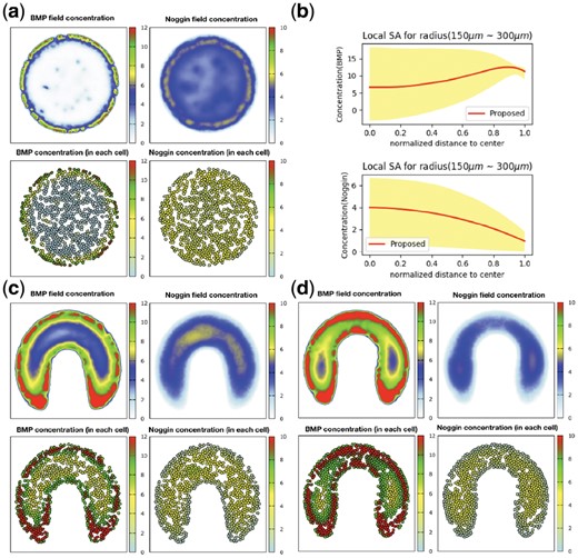
(a) Simulation on 3 mm colony. Increasing radius reveals spotty pattern. (b) Sensitivity of final pattern w.r.t. radius. Small changes in radius lead to significant effect on BMP and Noggin distributions in space. (c, d) Minor alternations in geometry in the real situation has made dramatic changes in the pattern. In the right figure, the bottleneck is slightly narrower than the left figure, leading to a significant change in the resulting pattern

3.5.2 Non-circular geometry

All the previous experiments have been done on circular confinement for colonies. Different geometries for colonies were considered and for each one simulation performed. We have shown the result of one geometry which resembles in-vivo gastrulation and left the others in the Supplementary (Fig. 6c and d). Based on simulations, our hypothesis about the high importance of geometry seems reasonable. By assuming each color as a separate fate, a small variation in curvature of geometry completely change the fate regions; but it needs an in vitro experiment for confirmation. We think it would be interesting to write state of the system or fate of each cell as a function of geometry or at least some features of geometry like curvature. It can be considered as future works, but for now, we have just performed some simulations on different geometries to clarify our claim.

Moreover, based on our observation, we can speculate that pattern formation initiates from the boundary (edge) of the colonies. BMP4 (Noggin) has the wave-like property, propagation of the wave initiates from the edge and gradually propagates toward the center of the colony. The final pattern formation is the direct consequence of interference between wave-like concentrations. Therefore, the edge plays a very critical role in the pattern formation.

4 Conclusions

We observed that cellular interaction plays an important role in pattern formation; to an extent that in absence of such interactions, the system exhibits time-course oscillatory behavior, while in presence of such interactions, the system shows stabilized behavior in time. Hence, the cellular interactions are among the pivotal factors that lead the system toward the desired pattern which is consistent with previous biological and experimental evidence. In addition, the colony diameter has a significant impact on the emerging pattern; increasing colony diameter can result in the formation of the spotty pattern, and our model also captures this behavior. Furthermore, we studied the effect of different parameters, and observed that some of them such as $r_1,\lambda ,D_B$ and D_N have greater impacts on final results. Subsequently, we scrutinized the effect of colony geometry on final pattern, and found out that as expected, even an incremental change in geometry can have a significant impact on the pattern. Experimental results are required to validate our observations.

Conflict of Interest: none declared.