Bayesian GWAS with Structured and Non-Local Priors

Abstract

Motivation

The flexibility of a Bayesian framework is promising for GWAS, but current approaches can benefit from more informative prior models. We introduce a novel Bayesian approach to GWAS, called Structured and Non-Local Priors (SNLPs) GWAS, that improves over existing methods in two important ways. First, we describe a model that allows for a marker’s gene-parent membership and other characteristics to influence its probability of association with an outcome. Second, we describe a non-local alternative model for differential minor allele rates at each marker, in which the null and alternative hypotheses have no common support.

Results

We employ a non-parametric model that allows for clustering of the genes in tandem with a regression model for marker-level covariates, and demonstrate how incorporating these additional characteristics can improve power. We further demonstrate that our non-local alternative model gives symmetric rates of convergence for the null and alternative hypotheses, whereas commonly used local alternative models have asymptotic rates that favor the alternative hypothesis over the null. We demonstrate the robustness and flexibility of our structured and non-local model for different data generating scenarios and signal-to-noise ratios. We apply our Bayesian GWAS method to single nucleotide polymorphisms data collected from a pool of Alzheimer’s disease and cognitively normal patients from the Alzheimer’s Database Neuroimaging Initiative.

Availability and implementation

R code to perform the SNLPs method is available at https://github.com/lockEF/BayesianScreening.

1 Introduction

Detecting associations between particularly influential genetic variants and a complex pathogenesis is of major interest within chronic disease research, and innovations in genome-wide association studies (GWAS) are desirable. A common practice in GWAS is massive univariate linear modeling, where each genetic marker (i.e. single nucleotide polymorphism, or SNP) is independently fit as a linear predictor to explain the variability in a given phenotype. Due to the large number of tests conducted in a genome-wide analysis (GWA), procedures that correct Type-I error rate cut-offs for multiple comparisons are commonly used. These strategies include controlling the family-wise error rate or false discovery rate (Benjamini and Hochberg, 1995; Holm, 1979; Hochberg and Tamhane, 1987). In GWAS, the massive number of tests requires a very stringent Type-I error rate correction. Kamboh et al. (2012) conducted a meta-analysis of GWAS on around 2.5 million SNPs with a Bonferroni correction to control family-wise error rate, and detected six SNPs associated with Alzheimer’s disease. Then, they mapped the critical values of each marker against the location of that marker on its corresponding gene (Kamboh et al., 2012). The location of the SNPs within a gene correlated with the significance level from their associated tests. This example suggests that a more informed data-dependent correction may yield increased power to detect marker-phenotype associations.

More contemporary research on multiple testing has incorporated a Bayesian perspective. Bayesian approaches to multiple testing follow two noticeable patterns: selection or shrinkage. Bayesian model selection uses posterior probabilities to select among different hypotheses given the data, and multiple testing can be treated with a hierarchical model on the prior probabilities for multiple related tests (Scott and Berger, 2010). Bayesian hierarchical modeling of effect sizes is similarly useful under multiple testing scenarios, by appropriately shrinking effects toward the null value. Bayesian hierarchical selection and shrinkage have both been considered in the GWAS context, and a key challenge is to incorporate additional characteristics for a more descriptive and powerful approach to multiple testing. These additional characteristics, such as the genomic position of a marker and its functional annotation, have been shown to influence a marker’s association with a given phenotype of interest (Kamboh et al., 2012; Lewinger et al., 2007; Zablocki et al., 2017). Yi et al. (2014) considered Bayesian model shrinking in the GWAS context and used additional marker level characteristics to influence the shrinkage of the parameters, and collected the few markers with high signal. Lewinger et al. (2007) introduced a fully Bayesian scheme for marker selection in which additional characteristics, such as SNP annotation, influence the prior probability of the null hypothesis for each marker. Alternatively, Zablocki et al. (2014) described a Bayesian framework that allows covariates to modulate a false discovery rate adjustment; Zablocki et al. (2017) followed up their work by relaxing distributional assumptions and uses B-splines for a more flexible modeling approach. Lock and Dunson (2017) described a hierarchical model in which the prior probability of association for a given marker depends on its parent gene, and the gene-level effects are modeled flexibly with a non-parametric Dirichlet Process (DP) prior. We build on this hierarchical DP structure in this work, to allow for clustering of the parent gene effect while also incorporating functional information on the markers.

For Bayesian model selection, results are often sensitive to the specification of priors under the null and alternative hypotheses, and thus these must be considered carefully. Classical frequentist hypotheses specifications often have a point null while the alternative is anything but that point null. However, in the Bayesian framework it is often the case that the null hypothesis is a point null while the alternative hypothesis is a more diffuse distribution. A local alternative prior includes the null in its support. It has been shown that the asymptotic rates of evidence in favor of either hypothesis differs exponentially under such a scenario (Johnson and Rossell, 2010; Lock and Dunson, 2015). Non-local priors (henceforth NLP) were introduced by Johnson and Rossell (2010, 2012) to resolve this issue with Bayesian alternative hypothesis specification, and they are commonly used for model selection in a regression context. The use of NLPs in GWAS for multivariate regression modeling and a continuous outcome was explored by Sanyal et al. (2019). We introduce a NLP for two-sample tests with categorical data that is appropriate for GWAS screening studies. NLPs are sensitive to user-specified hyperparameters, and in this article we explore the influence of these hyperparameters and propose a method of marginal likelihood maximization to select the hyperparameters in our context.

Our primary methodological contributions are twofold: (i) to incorporate prior knowledge on markers to estimate probabilities of phenotype associations more accurately and improve interpretation, and (ii) to introduce a NLP model for the two-sample testing context for Bayesian GWAS applications. For (i), we build on Lock and Dunson (2017) and extend the non-parametric Bayesian method for parent-gene clustering to incorporate additive effects for additional marker-level data. For (ii), we use a probit link function to model the difference in minor allele rates between two samples via a NLP. We describe extensive simulation studies to assess both contributions, demonstrating improved performance while also highlighting caveats in their implementation. Lastly, we illustrate our proposed model on the SNP level data from the Alzheimer’s Disease Neuroimaging Initiative (ADNI) and discuss the SNPs and genes that are found to be associated with Alzheimer’s disease (www.adni-info.org).

2 Model

2.1 GWA modeling framework

In this section we describe our general framework for Bayesian GWAS and discuss our contributions. There are many different forms of genetic marker data, however, we focus on the minor allele proportion of presence (either one or two minor alleles present) for given SNPs (henceforth minor allele rates). The SNPs may be grouped by the gene region that they fall within (i.e. their gene-parent). We consider the common scenario of screening for markers that are associated with the lack of or presence of a given phenotype (represented by 0 and 1, respectively). Denote $N_{\mathit{ij}}^0$ and $N_{\mathit{ij}}^1$ as the total number of control and case study participants, respectively, for genetic marker j within parent i. Denote the number of individuals with the minor allele present in each group as $s_{\mathit{ij}}^0$ and $s_{\mathit{ij}}^1$⁠, which follow a binomial distribution with underlying minor allele rates $p_{\mathit{ij}}^0$ and $p_{\mathit{ij}}^1$⁠, respectively, as opposed to the minor allele frequencies. That is,

$$s_{\mathit{ij}}^0\sim \text{Bin}(N_{\mathit{ij}}^0,p_{\mathit{ij}}^0)\hspace{0.17em}\hspace{0.17em}\text{and}\hspace{0.17em}\hspace{0.17em}{s}_{\mathit{ij}}^1\sim \text{Bin}(N_{\mathit{ij}}^1,p_{\mathit{ij}}^1),$$

where $\text{Bin}(n,p)$ denotes the Binomial distribution with total count parameter n and probability of success p. We specify null and alternative hypotheses, $H_{\mathit{ij}}^0$ and $H_{\mathit{ij}}^A$⁠, that define prior models for $p_{\mathit{ij}}^0$ and $p_{\mathit{ij}}^1$⁠. Then the marginal likelihoods under each hypothesis can be used to find the posterior probability of association for each marker. Let π_ij be the prior probability of $H_{\mathit{ij}}^A$⁠, then

$$\begin{array}{c}P(H_{\mathit{ij}}^A|s_{\mathit{ij}}^0,s_{\mathit{ij}}^1)=\\ \frac{{\pi }_{\mathit{ij}}·P(s_{\mathit{ij}}^0,s_{\mathit{ij}}^1|H_{\mathit{ij}}^A)}{{\pi }_{\mathit{ij}}·P(s_{\mathit{ij}}^0,s_{\mathit{ij}}^1|H_{\mathit{ij}}^A)+(1-{\pi }_{\mathit{ij}})·P(s_{\mathit{ij}}^0,s_{\mathit{ij}}^1|H_{\mathit{ij}}^0)}\end{array}$$

(1)

where $P(s_{\mathit{ij}}^0,s_{\mathit{ij}}^1|H_{\mathit{ij}}^0)$ and $P(s_{\mathit{ij}}^0,s_{\mathit{ij}}^1|H_{\mathit{ij}}^A)$ refer to the marginal likelihood under the null and alternative hypotheses for marker j within parent i, respectively. If there is not prior information on the SNPs then π_ij has been set to 0.5, reflecting that either hypothesis has 50% of being true a priori (Stephens and Balding, 2009).

In Section 2.2 we discuss implementing non-local priors for the likelihoods under $H_{\mathit{ij}}^0$ and $H_{\mathit{ij}}^A$ in Equation (1). In Section 2.3 we elaborate on using a structured model for π_ij in Equation (1) that incorporates marker-level covariates and the parent gene of each marker.

2.2 Incorporating non-local hypotheses

In our model we incorporate the non-local prior to enforce dissimilarity in a genetic marker’s minor allele rates between the patient classes, under the alternative hypothesis. Under $H_{\mathit{ij}}^0$⁠: $p_{\mathit{ij}}^0=p_{\mathit{ij}}^1=p_{\mathit{ij}}\sim U(0,1)$⁠, that is, we assume that the probability of a minor allele is the same for both groups, with a uniform prior over the unit interval. Under $H_{\mathit{ij}}^A$⁠: $p_{\mathit{ij}}^0=\Phi ({\alpha }_{0ij}-{\alpha }_{1ij}),$$p_{\mathit{ij}}^1=\Phi ({\alpha }_{0ij}+{\alpha }_{1ij})$⁠, where ${\alpha }_{0ij}\sim N(0,1)$ and ${\alpha }_{1ij}\sim \mathit{NLP}(\tau ,k,v)$ where

$$\mathit{NLP}({\alpha }_1|\tau ,k,v)=\frac{k{\tau }^{v/2}}{\Gamma (v/2k)}{[{\alpha }_1^{\mathrm{2}}]}^{-(v+1)/2}\hspace{0.17em}\text{exp}[-{\left(\frac{{({\alpha }_1)}^2}{\tau }\right)}^{-k}].$$

(2)

Here, $\Phi$ denotes the cumulative distribution function of a standard normal distribution while $N(·,·)$ means the Normal distribution with a mean and a variance parameter, respectively. Note that if hypothetically ${\alpha }_{1ij}=0$⁠, then the alternative model is equivalent to the null. However, ${\alpha }_{1ij}=0$ is not within the support of the prior; this is the key characteristic of the non-local prior as it enforces $p_{\mathit{ij}}^0$ and $p_{\mathit{ij}}^1$ to be unequal. The specification of the hyperparameters $\{\tau ,k,v\}$ is discussed in Section 3.2.1.

To our knowledge, there has not been an investigation of non-local priors within our context. However, non-local alternative priors generally yield exponential rates of convergence toward a true null or true alternative (Johnson and Rossell, 2010), whereas local alternative priors do not. We verify this with a simple simulation study in Section 4.3.

In addition to the non-local alternative model, we consider a straightforward local model following Stephens and Balding (2009). Under $H_{\mathit{ij}}^0:p_{\mathit{ij}}^0=p_{\mathit{ij}}^1=p_{\mathit{ij}}\sim U(0,1)$ and under $H_{\mathit{ij}}^A:p_{\mathit{ij}}^0\sim \mathrm{U}(0,1)$ and $p_{\mathit{ij}}^1\sim U(0,1)$ are treated independently. Although $p_{\mathit{ij}}^1$ and $p_{\mathit{ij}}^0$ are independent under the alternative, the alternative still supports the possibility that $p_{\mathit{ij}}^0=p_{\mathit{ij}}^1$⁠, which is consistent with the null hypothesis. This is the key distinction between the local and non-local models; the former does not explicitly enforce inequality while the latter does. The marginal likelihoods under the null and local alternative have closed forms and are supplied in Section 3.1.

2.2.1 Exploring the non-local density

Here we investigate the implication of the hyperparameter settings for the non-local density on the magnitude of the difference in minor allele rates between classes. First, recall that $\Phi ({\alpha }_0-{\alpha }_1)=p^0$ and $\Phi ({\alpha }_0+{\alpha }_1)=p^1$⁠, and thus ${\alpha }_1=\frac{1}{2}({\Phi }^{-1}(p^1)-{\Phi }^{-1}(p^0))$⁠. This provides a natural point of comparison to the local model, wherein the minor allele rates p⁰ and p¹ follow independent U(0, 1) distributions; under these assumptions, ${\alpha }_1=\frac{1}{2}({\Phi }^{-1}(p^1)-{\Phi }^{-1}(p^0))\sim N(0,\frac{1}{2})$⁠. Figure 1 shows the density for α₁ under different specifications of the non-local alternative prior, and for the local alternative. The value of τ largely controls the range of support for the non-local prior and the size of the ‘gap’ with negligible density near 0; the value of V controls the variability near the boundaries of this gap. As τ changes but is rather small, the density of the non-local parameter α₁ also substantially changes. In comparison, the local model is rather diffuse over this support. The effect of the hyperparameters in the non-local density illustrate the sensitivity to the values of τ and V, and we caution against arbitrarily selecting their values. We devised a likelihood maximization scheme, described in Section 3.2.1, to empirically nominate a candidate set of values V, τ and k.

Fig. 1.

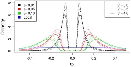
Non-local densities with varying parameter values V and small τ with k = 1. The distribution for α₁ under the local alternative hypothesis is provided for comparison

2.3 Incorporating structured dependence

Here we describe our approach to incorporate genomic structure and prior information to infer π_ij in Equation (1). Our approach generalizes to any constructed likelihood per marker under each hypothesis, $P(s_{\mathit{ij}}^0,s_{\mathit{ij}}^1|H_{\mathit{ij}}^0)$ and $P(s_{\mathit{ij}}^0,s_{\mathit{ij}}^1|H_{\mathit{ij}}^A)$⁠, such as those in Section 2.2. Let $\mathbf{X}=[X_{\beta },X_{\theta }]$ be a design matrix of additional prior data for each marker. In our context, $X_{\beta }$ includes categorical indicators giving the functional classification for each SNP, and $X_{\theta }$ is a gene-parent affiliation matrix (i.e. an ANOVA design matrix of gene affiliation for each SNP) and $\Theta =[\beta ,\theta ]$⁠. We use a probit link to model the marker prior probabilities as a function of covariates: ${\pi }_{\mathit{ij}}=\Phi (x_{\mathit{ij}}^T\Theta )$⁠, where $\Phi$ is the standard normal CDF. We place a N(0, 1) prior on the coefficients β. For the gene-level effects θ_i, we use a flexible Dirichlet process prior with concentration parameter α and a N(0, 1) base distribution. We denote this distribution using the stick-breaking construction: $\omega |\alpha \sim \mathit{GEM}(\alpha ),\hspace{0.17em}{\varphi }_k\stackrel{i.i.d}{\sim }N(0,1)$⁠, with $S_i|\omega \sim \text{Mult}(\omega )$ and ${\theta }_i|S_i,\{{\varphi }_k\}\sim F({\varphi }_{k_i})$⁠, where $\text{Mult}(·)$ denotes the multinomial distribution, and GEM is the distribution for the stick-breaking construction of a Dirichlet process with concentration parameter α (Pitman et al., 2002). To flexibly infer the concentration of the gene effects we use a $\Gamma (a,b)$ prior on α, where $\Gamma (\alpha ,\beta )$ is the gamma distribution with shape and scale parameters α and β. We set $a=b=1.1$ for these hyperparameters. Lastly, we truncate the number of stick-breaks for the DP model at 20 (Sethuraman, 1994).

We point out certain aspects of our model that build off existing work on covariate modulated prior probabilities for GWAS. Without gene-level effects (⁠$\theta =0$⁠) our model is analogous to that in Lewinger et al. (2007), who used a logit rather than a probit link for the prior probabilities π_ij. We used a probit link primarily to facilitate efficient posterior computation (see Section 3.2). Moreover, without additional marker level covariates (⁠$\beta =0$⁠), our model is analogous to that in Lock and Dunson (2017), who used a Dirichlet process prior with U(0, 1) base distribution to model gene-level posterior probabilities. As U(0, 1) is equivalent to a N(0, 1) distribution with a probit link, we have directly extended the gene-level model of Lock and Dunson (2017) to allow for additional marker covariates.

3 Estimation

3.1 Marginal likelihood estimation

Under the null hypothesis for the non-local and local models of Section 2.2 the marginal likelihood is

$$P(s_{\mathit{ij}}^0,s_{\mathit{ij}}^1|H_{\mathit{ij}}^0)=\beta (1+s_{\mathit{ij}}^1+s_{\mathit{ij}}^0,1+s_{\mathit{ma},\mathit{ij}}^1+s_{\mathit{ma},\mathit{ij}}^0)\left(\begin{array}{c}{N}_{\mathit{ij}}^0\\ s_{\mathit{ij}}^0\end{array}\right)\left(\begin{array}{c}{N}_{\mathit{ij}}^1\\ s_{\mathit{ij}}^1\end{array}\right),$$

where $\beta (·,·)$ denotes the Beta coefficient, and the subscript ma denotes major allele count: $s_{\mathit{ma},\mathit{ij}}^0=N_{\mathit{ij}}^0-s_{\mathit{ij}}^0$ and $s_{\mathit{ma},\mathit{ij}}^1=N_{\mathit{ij}}^1-s_{\mathit{ij}}^1$⁠. The marginal likelihood under the alternative hypothesis for the local model is also calculated directly:

$$\begin{array}{c}P(s_{\mathit{ij}}^0,s_{\mathit{ij}}^1|H_{\mathit{ij}}^A)=\hfill \\ \beta (1+s_{\mathit{ij}}^1,1+s_{\mathit{ma},\mathit{ij}}^1)\beta (1+s_{\mathit{ij}}^0,1+s_{\mathit{ma},\mathit{ij}}^0)\left(\begin{array}{c}{N}_{\mathit{ij}}^0\\ s_{\mathit{ij}}^0\end{array}\right)\left(\begin{array}{c}{N}_{\mathit{ij}}^1\\ s_{\mathit{ij}}^1\end{array}\right).\end{array}$$

Under the non-local alternative the marginal likelihood is

$$P(s_{\mathit{ij}}^0,s_{\mathit{ij}}^1|H_{\mathit{ij}}^A)=\int \int \text{Bin}(s_{\mathit{ij}}^0;N_{\mathit{ij}}^0,p_{\mathit{ij}}^0)·\text{Bin}(s_{\mathit{ij}}^1;N_{\mathit{ij}}^1,p_{\mathit{ij}}^1)$$

$$·N({\alpha }_{0ij};0,1)·\mathit{NLP}({\alpha }_{1ij};\tau ,v,k)\partial {\alpha }_{0ij}\partial {\alpha }_{1ij},$$

where $p_{\mathit{ij}}^0=\Phi ({\alpha }_{0ij}-{\alpha }_{1ij})$ and $p_{\mathit{ij}}^1=\Phi ({\alpha }_{0ij}+{\alpha }_{1ij})$⁠. We compute this intractable integral via a two-step Monte Carlo approach. First, we generate T values for each of α₀ and α₁ from their prior; that is, we generate α₀ from a N(0, 1) distribution, and α₁ from the specified NLP via a Metropolis-Hastings approach. For each simulated pair $({\alpha }_0^{(t)},{\alpha }_1^{(t)})$ we compute $p^{0(t)}=\Phi ({\alpha }_0^{(t)}-{\alpha }_1^{(t)})$ and $p_{\mathit{ij}}^{1(t)}=\Phi ({\alpha }_0^{(t)}+{\alpha }_1^{(t)})$⁠, and approximate the marginal likelihood empirically:

$$P(s_{\mathit{ij}}^0,s_{\mathit{ij}}^1|H_{\mathit{ij}}^A)\approx \frac{1}{T}\sum _{t=1}^T\text{Bin}(s_{\mathit{ij}}^0;N_{\mathit{ij}}^0,p^{0(t)})·\text{Bin}(s_{\mathit{ij}}^1;N_{\mathit{ij}}^1,p^{1(t)}).$$

3.2 Posterior estimation

We compute the full posterior under the structured prior using a Gibbs sampling approach, with a latent variable augmentation for the probit link as described in Albert and Chib (1993). That is, we introduce Z_ij as latent variables that depend on the model indicators Y_ij: $Z_{\mathit{ij}}\sim N(x_{\mathit{ij}}^T\Theta ,1)$ with $x_{\mathit{ij}}^T\Theta =x_{\mathit{ij}}^T\beta +{\theta }_i$⁠, where Y_ij = 1 if Z_ij > 0 and Y_ij = 0 otherwise. To sample from the DP model on the gene effects we use its stick-breaking construction (Sethuraman, 1994), and sample from the full conditionals as described in Dunson (2010). The full Gibbs sampling scheme proceeds as follows:

• (1) Designate Alternative Markers:

The prior probability of association for marker j within parent i is

$${\pi }_{\mathit{ij}}=\Phi ({\mathbf{x}}_{\mathbf{i}\mathbf{j}}^T\Theta )\hspace{0.17em}\hspace{0.17em}\hspace{0.17em}\text{and}\hspace{0.17em}\hspace{0.17em}\Phi \hspace{0.17em}\hspace{0.17em}\text{is} \text{the} \text{Normal} \text{CDF}.$$

Then the posterior probability of association is

$$P(H_{\mathit{ij}}^A|s_{\mathit{ij}}^0,s_{\mathit{ij}}^1)=\frac{{\pi }_{\mathit{ij}}P(s_{\mathit{ij}}^0,s_{\mathit{ij}}^1|H_{\mathit{ij}}^A)}{{\pi }_{\mathit{ij}}P(s_{\mathit{ij}}^0,s_{\mathit{ij}}^1|H_{\mathit{ij}}^A)+(1-{\pi }_{\mathit{ij}})P(s_{\mathit{ij}}^0,s_{\mathit{ij}}^1|H_{\mathit{ij}}^0)}$$

and $\hspace{0.17em}{Y}_{\mathit{ij}}\sim \text{Bern}(P(H_{\mathit{ij}}^A|s_{\mathit{ij}}^0,s_{\mathit{ij}}^1)).$

• (2) Update DP parameters for$\theta \prime$⁠:

(A) First we allocate each gene-parent effect θ_i to one of the DP atoms h, denoted by $S_i=h$⁠, from a closed form multinomial conditional posterior with probabilities:

$$\begin{array}{c}Pr(S_i=h|-)=\hfill \\ \frac{\{V_h{\Pi }_{l<h}(1-V_l)\}{\prod }_j^{n_i}N(Z_{\mathit{ij}}-x_{(\beta )\mathit{ij}}^T\beta ;\theta {\prime }_h,1)}{{\sum }_{r=1}^H\{V_r{\Pi }_{s<r}(1-V_s)\}{\prod }_j^{n_i}N(Z_{\mathit{ij}}-x_{(\beta )\mathit{ij}}^T\beta ;\theta {\prime }_r,1)},\end{array}$$

where $h=1,\dots ,H$⁠, n_i are the number of markers assigned to gene i, ${\theta }_h^{\prime }$ is the effect for atom h and H is the number of stick-breaks.

(B) We update the stick-breaking weights from the conjugate posterior distribution:

$$(V_h|-)\stackrel{\mathit{ind}}{\sim }\text{Beta}(1+\sum _{i=1}^{G}I(S_i=h),\alpha +\sum _{i=1}^{G}I(S_i>h)),$$

where I(A) is the indicator function (if A is true then I(A) = 1, and I(A) = 0 otherwise), G is the number of genes and V_H = 1.

(C) Update the DP atoms (random intercepts for each cluster) by sampling from their Normal posteriors

$$\begin{array}{c}({\theta }_h|-)\stackrel{\mathit{ind}}{\sim }\hfill \\ N(\frac{1+\sum _{i:S_i=h}{\sum }_{j=1}^{n_i}{Z}_{\mathit{ij}}-x_{(\beta )\mathit{ij}}^T\beta }{1+\sum _{i:S_i=h}{n}_i},\frac{1}{1+\sum _{i:S_i=h}{n}_i}).\end{array}$$

(D) Reassign ${\theta }_i=\theta {\prime }_{S_i}$⁠.

• (3) Update DP concentration α via a Metropolis-Hastings step with a $\Gamma (1.1,1.1)$ prior.

• (4) Update additional regression parameters β via

  $$(\beta |-)\sim N(\widehat{\beta },{(I_{\beta }+X_{\beta }^{\prime }{X}_{\beta })}^{-1})$$

where $\widehat{\beta }$ is the conditional posterior mean

$$\widehat{\beta }={(I_{\beta }+X_{\beta }^{\prime }{X}_{\beta })}^{-1}{X}_{\beta }^{\prime }(Z-X_{\theta }\theta ).$$

• (5) Update Latent Variable Z by a truncated normal distribution depending on Y_ij.

  $$Z_{\mathit{ij}}\sim N^{+}({\mathbf{x}}_{\mathbf{i}\mathbf{j}}^T\Theta ,1)\hspace{0.17em}\hspace{0.17em}\text{if}\hspace{0.17em}\hspace{0.17em}\hspace{0.17em}{Y}_{\mathit{ij}}=1;\hspace{0.17em}\hspace{0.17em}\hspace{0.17em}{Z}_{\mathit{ij}}\sim N^{-}({\mathbf{x}}_{\mathbf{i}\mathbf{j}}^T\Theta ,1)\hspace{0.17em}\hspace{0.17em}\hspace{0.17em}\text{if}\hspace{0.17em}\hspace{0.17em}\hspace{0.17em}{Y}_{\mathit{ij}}=0,$$

  where $N^{+}(·)$ and $N^{-}(·)$ refer to truncated from the left and right at 0, respectively.

We take the mean over Gibbs samples to obtain point estimates for model parameters and to obtain the posterior probability of association for each marker.

3.2.1 Log-marginal likelihood maximization for non-local parameter determination

We select the non-local alternative hyperparameters for given data through a computationally efficient marginal likelihood empirical maximization technique. Given a dataset, we compute the marginal likelihoods under the null and alternative hypotheses for each marker, as explained in Section 3.1. Then we designate for marker ij, $I(H_{\mathit{ij}}^A)=1$ if $P(s_{\mathit{ij}}^0,s_{\mathit{ij}}^1|H_{\mathit{ij}}^A)>P(s_{\mathit{ij}}^0,s_{\mathit{ij}}^1|H_{\mathit{ij}}^0)$⁠, and $I(H_{\mathit{ij}}^A)=0$ otherwise. The likelihood for all markers is computed as

$$P(s_{\mathit{ij}}^0,s_{\mathit{ij}}^1)=P(s_{\mathit{ij}}^0,s_{\mathit{ij}}^1|H_{\mathit{ij}}^A)I(H_{\mathit{ij}}^A)+P(s_{\mathit{ij}}^0,s_{\mathit{ij}}^1|H_{\mathit{ij}}^0)(1-I(H_{\mathit{ij}}^A))$$

(3)

We then take the average of log-likelihood over all markers, given the NLP parameters. We evaluate this expression over a grid of V and τ values while holding k = 1, and the pair of NLP parameters yielding the highest average of the log-likelihood is the chosen set of parameters for the subsequent full analysis that incorporates the hierarchical estimation of the prior probability of association.

4 Simulation studies

4.1 Structured prior: gene-parent effects only

Here we describe a simulation study in which the prior probability that a marker is associated with a given phenotype depends on its gene-parent. We consider several scenarios, with varying levels of sparsity in the number of associated markers and the gene structure. We design our simulation studies to explore the performance of our proposed method with respect to these different levels of association. Namely, we consider four cases where the prior probabilities are drawn from (i) an all null distribution, (ii) a bimodal distribution in which 80% of genes have no association and the markers in the remaining 20% are all associated, (iii) a Beta$(0.2,1)$ distribution for parent prior probabilities and (iv) a uniform distribution for the parent prior probabilities. For each scenario, we simulate data according to the local model in Section 2.2, with 100 case and control samples each (⁠$N^0=N^1=100$⁠), 500 parent genes, and the number of markers for each gene uniformly generated between 2 and 30.

Under each scenario, we compare three structured prior models: (i) our proposed hierarchical DP model, (ii) a separate model where parent level effects are modeled separately with independent N(0, 1) distributions (i.e. the parent probabilities are independent U(0, 1) after probit transformation) and (3) a joint model where all markers share the same prior probability, irrespective of their parent gene, with a U(0, 1) prior on this probability.

Table 1 gives the mean absolute error (MAE) for the inferred gene-level probabilities and the marker-level posterior probabilities for each scenario. Our hierarchical DP model outperforms the separate and joint approaches for the Beta$(1,0.2)$ and Bimodal scenarios. The Uniform generative model matches the separate inference model, however, the results for the DP model are comparable to the separate model under this scenario and both substantially outperform the joint model. Similarly, the joint model is appropriate for the All null case because all parent genes have the same signal, yet the DP model is again comparable while substantially outperforming the separate model. Together, these scenarios reflect the advantages of implementing a flexible prior that accommodates different distributions of parent-gene effects, such as the DP. Moreover, the difference in the marker MAEs illustrate how a well-specified prior for the parent-gene effects can lead to more accurate posterior probabilities for the markers.

Table 1.

Mean absolute error (MAE) in gene parent probabilities, and marker posterior probabilities, for four different simulation scenarios and three models for the marker prior probabilities

	All null	Bimodal	Beta(0.2, 1)	Uniform
Parent MAE
DP	0.0002	0.0011	0.0705	0.1196
Separate	0.1085	0.1220	0.1101	0.1176
Joint	0.0003	0.3150	0.1870	0.2587
Marker MAE
DP	0.0008	0.0193	0.0531	0.1531
Separate	0.0286	0.0487	0.0697	0.1531
Joint	0.0004	0.1151	0.0762	0.2052

4.2 Structured prior: gene-parent and covariate effects

We evaluate the addition of covariates in the hierarchical setting by simulating true marker associations that are influenced by the assigned gene-parents as well as six additional covariates (six categorical variables that reflect SNP annotation). We simulated data as in the Uniform scenario of Section 4.1, but with $\Gamma (2,1)$ effects for the six additional marker-level variables. We perform 20 replications of the simulation, and we compare our model with covariates to the same model with covariate effects set to 0. In the cases considered above, we estimate Bayesian credible interval coverage of the parent and covariate effects (when applicable) and mean absolute error (MAE) in marker posterior probability for comparing models under similar data settings. All simulations are done with 2000 collected samples with 1000 burn-in for convergence to the posterior distributions.

When gene effects are drawn from a standard normal distribution, the addition of marker-level covariates lowered MAE in marker posterior probability by about 0.03 (Table 2). We highlight that under similar circumstances, for a model that is misspecified when covariates truly contributed to posterior probabilities of marker association, the MAE of that model was around 0.1719. Coverage for gene-parent effects were less than the nominal under either setting. This likely reflects the discrepancy of the generative model (with independent and distinct gene effects) and our DP model (which assumes some clustering of the genes). However, as shown in Section 4.1, the accuracy of the results under the DP model is comparable to those under the generative model. We did not explore the estimation accuracy of our model for continuous marker-level covariates.

Table 2.

Adding covariates with parent hierarchical structure: the model with local priors

Number of markers	Number of genes
	500	1000
	Parent with 6 categorical effects
15	0.1363 ± 0.0043	0.1389 ± 0.0030
30	0.1348 ± 0.0033	0.1316 ± 0.0042
50	0.1259 ± 0.0027	0.1281 ± 0.0038
	Parent effects only
15	0.1642 ± 0.0012	0.1625 ± 0.0006
30	0.1551 ± 0.0009	0.1552 ± 0.0006
50	0.1518 ± 0.0010	0.1512 ± 0.0004

Note: The true parent effects are drawn from a N(0, 1). True categorical effects are drawn from a $\Gamma (2,1)$ distribution. Each model is applied to simulated data with matching data generation specifications (with and without 6 categorical effects, respectively). These measures are mean absolute errors over 20 simulations ± their standard errors.

4.3 Non-local alternative: asymptotic rates

We generate p⁰ and p¹ under either the null model or the non-local alternative model, and generate data s⁰ and s¹ for a specified sample size $N^0=N^1=N$⁠. We calculate marginal likelihoods under each hypothesis via importance sampling (see Section 3.1). Figure 2 shows the log Bayes factors for increasing sample size N, demonstrative of exponential convergence under both the null and the alternative.

Fig. 2.

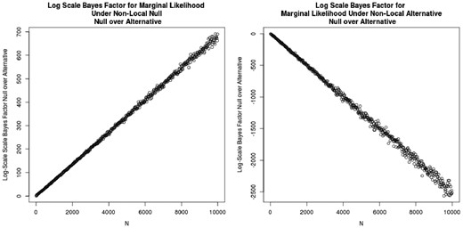
Non-local prior and asymptotic rates of convergence: Data were generated with non-local parameters $\mathbf{\tau }=2,\hspace{0.17em}\mathbf{V}=4$ and $\mathbf{k}=1$⁠.

4.4 Non-local alternative: sensitivity and comparison

To evaluate the non-local alternative model, we simulate data as in the Uniform scenario of Section 4.1, but using the non-local alternative of Section 2.2 to generate minor allele counts. As potential hyperparameters for the non-local model, we consider all possible combinations of the values $V:\{2.0,2.50,3.0,3.50,4.0\}$ and $\tau :\{0.10,0.45,0.80,1.15,1.50\}$⁠, with k = 1, For estimation we also consider the same parameter combinations for the non-local model, as well as the local alternative model. We collect the 80% and 90% credible coverage and the mean absolute error in marker posterior probability of association for twenty simulations of each scenario.

Figure 3 displays the marker MAE for each generative scenario and for each estimation model. The results show that the non-local alternative generally performs substantially better when the true generative model is non-local, even if the hyperparameters are misspecified. For $\tau =0.10$ and 0.45, τ reflects possible effect sizes in associated probabilities, before transforming to the probit scale. Most often, for data generated with $\tau =0.10$⁠, the model with the specified $\widehat{\tau }=0.10$ outperforms models that use other values for $\widehat{\tau }$ with respect to mean absolute error. This pattern is also exhibited with $\tau =0.45$ for the data and the specified model parameter. However, our model exhibits a flip in performance once the true τ is large enough, when the true τ changes from 0.10 to 0.45. For the case that the data were truly generated from an NLP distribution with τ larger than 0.45, the local model performs consistently worse than the non-local model. This reflects that larger τ values imply easier detection of associated markers by the non-local prior, as V and τ can be viewed as a joint effect size modulator for the difference between $p_{\mathit{ij}}^0$ and $p_{\mathit{ij}}^1$ (See Equation 2). As V grows and τ shrinks, we approach a scenario where there is little difference between $p_{\mathit{ij}}^0$ and $p_{\mathit{ij}}^1$⁠, thus approaching the behavior of the model specified under the local prior. With smaller values of V, the model not considering non-local priors improved slightly in terms of the three aforementioned statistics for true τ set at its smallest value.

Fig. 3.

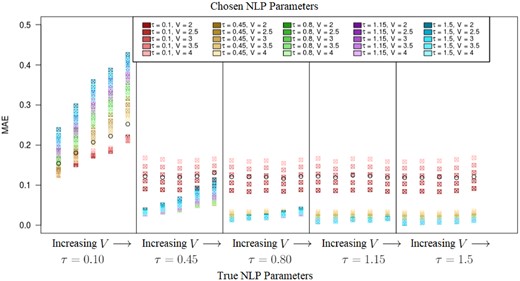
Non-local model implemented on non-local data: Mean Absolute Error (MAE) is shown for each pair of the parameter settings that generated the data and the parameter specifications for the model, V = $\{2.0,2.5,3.0,3.5,4.0\}$ and τ = $\{0.10,0.45,0.80,1.15,1.50\}$⁠. The $°$ refers to the results from the Local Model for comparison

We also consider the robustness of the non-local alternative prior when data are generated under the local model. The resulting MAE for marker posterior probabilities under different specifications of the non-local prior are shown in Table 3. The non-local prior gave comparable performance to the (correctly specified) local prior, under certain values of its hyperparameters, demonstrating the robustness of the non-local model even when the generative distribution under the alternative does not have a non-local density.

Table 3.

Non-local prior implemented on local generated data: MAE for marker posterior probabilities are shown for non-local prior specifications V and τ

τ / V	2.0	2.5	3.0	3.5	4.0
0.10	0.1508	0.1565	0.1636	0.1717	0.1809
0.45	0.1582	0.1548	0.1520	0.1499	0.1481
0.80	0.1751	0.1710	0.1669	0.1639	0.1607
1.15	0.1887	0.1840	0.1799	0.1762	0.1728
1.50	0.2002	0.1943	0.1908	0.1871	0.1831

Note: The local model had a MAE of 0.1551.

4.5 Non-local alternative: hyperparameter selection

We evaluate our marginal likelihood maximization technique to determine the true set of hyperparameters for the NLP. First, we generate data with half of the markers from the null and half of the markers from a non-local alternative, with 15 000 total markers, $N^0=100$ controls and $N^1=100$ cases. After generative data, we empirically estimate the NLP parameters as described in Section 3.2.1. We ran 30 simulations for each combination of: V: 2.0, 2.50, 3.0, 3.50, 4.0; τ: 0.10, 0.45, 0.80, 1.15, 1.50; and k = 1, for data generation and modeling.

The proposed log-likelihood maximization method detected the appropriate set of parameters in most of the cases over the thirty simulations (see Table 4). τ is accurately estimated in most of the simulations; smaller values of τ are estimated to be the true value more often than for larger values of τ. This reflects that the degree to which the case and control proportions of minor allele presence differ can be quite small and be estimated quite accurately for this method. In general, the estimated values for $\widehat{V}$ were less accurate, but still tended to be correct in a majority of simulations.

Table 4.

Non-local prior parameter selection results

V / τ	0.10	0.45	0.80	1.15	1.50
(a)
2.0	90.00%	93.33%	76.67%	60.00%	76.67%
2.5	33.33%	83.33%	86.67%	76.67%	56.67%
3.0	10.00%	80.00%	80.00%	76.67%	80.00%
3.5	6.66%	80.00%	86.67%	70.00%	80.00%
4.0	0.00%	70.00%	83.33%	80.00%	83.33%
(b)
τ /  $\widehat{\tau }$	0.10	0.45	0.80	1.15	1.50
0.10	147	3	0	0	0
0.45	0	145	5	0	0
0.80	0	2	134	14	0
1.15	0	0	2	123	25
1.50	0	0	0	22	128
(c)
V /  $\widehat{V}$	2.0	2.5	3.0	3.5	4.0
2.0	124	21	2	0	3
2.5	34	92	11	2	1
3.0	30	3	98	10	5
3.5	0	8	39	97	6
4.0	0	1	12	42	95

Note: (a) Percentages for the log-likelihood maximization technique correctly specifying the non-local parameter values V and τ for the data generation out of 30 simulations for each scenario. (b) Total counts specifying τ correctly and incorrectly; rows and columns correspond to true and chosen τ, respectively. (c) Total counts specifying V correctly and incorrectly; rows and columns correspond to true and chosen V, respectively.

5 Application to ADNI data

The Alzheimer’s Disease Neuroimaging Initiative is a multi-center effort in identifying genomic, metabolomic, and neurological markers that associate with Alzheimer’s disease progression. We obtained our samples from the ADNI1 period of this initiative. These samples were genotyped using the Illumina Human610-Quad BeadChip and GenomeStudio v2009.1 was used to process the intensity data (www.adni-info.org). We collected 584 994 SNPs without functional annotation from 179 patients with Alzheimer’s disease (AD) and 214 with cognitively normal status (CN). Then we used the BioMart package in R version 3.4.1, to gather marker consequences and gene assignments for each SNP (R Core Team, 2017). We omitted SNPs that had duplicate entries to rid of the ambiguity in gene and marker consequence assignments. The counts of SNP consequence categories are: 77 splice cites, 497 5′UTR, 4861 3′UTR, 3324 non-synonymous, 1716 synonymous and 267 550 introns. We omitted intergenic SNPs from this analysis. There are 18 957 unique genes for 278 025 SNPs, and we apply our model onto this data. For up-to-date information, please go to adni.loni.usc.edu.

We applied our proposed hierarchical gene-parent and marker-level covariate adjusted model with non-local priors to the 278 025 SNPs from ADNI to identify markers that have high posterior probability of association with AD. From the SNP annotations collected from BioMart, we created an ANOVA-like binary matrix for SNP annotation (i.e. synonymous, intronic, etc.). For our analysis, we designated intronic SNPs as the reference group. We applied our maximum log-likelihood strategy to determine the optimal set of non-local prior parameters to model the ADNI data. We evaluated the mean log-likelihoods of the data over a large grid of values for τ and V, where $\tau :0.001,0.01,0.05,0.075,0.1,0.2,0.45,0.8,1.15,1.5$ and $V:2,3,4,5,6,7,8,9,10$⁠. Following this procedure, we analyzed the ADNI data with our hierarchical model that employs the previously determined NLP parameters in the alternative marginal likelihood estimation. 20 000 samples of each of the parameters and the posterior probability of association for markers were collected after a burn-in of 10 000 samples.

The maximum log-likelihood strategy for choosing the optimal set of non-local parameters yielded $\widehat{V}=8$ and $\widehat{\tau }=0.075$⁠, with a mean log-likelihood of −8.23; in comparison, the local model resulted in a mean log-likelihood of −8.35. Under our chosen non-local specification, the top SNP was rs2075650 with a posterior probability of association of 88.14% [see Table 5a for all detected SNPs with a PPA of at least 10%]. This SNP is located on TOMM40, near APOE4; this is a gene repeatedly observed to be significantly associated with Alzheimer’s disease in GWA studies. In comparison, not one SNP is identified when using Fisher’s exact test with the various multiple testing corrections. We only report rs2075650 as a significant marker with a modest expected false discovery rate, and a Holm adjusted P-value cut-off smaller than 10%. The flexible prior on the marker-gene membership yielded uniform atom-effect convergence to one or two values around −3.3 over the collected samples. This reflects that the probability of a random SNP within a given gene being associated with Alzheimer’s disease is very small. SNP annotation effects are summarized in Table 5b. Within Table 5a we include the difference in proportions of minor allele presence between the case and controls calculated from the raw data. These values may provide guidance on how to interpret one SNP’s relationship with Alzheimer’s disease. For instance, rs2075650 has the highest probability of association and has a positive risk difference, meaning there were more cases annotated with minor allele presence, 1 or 2 minor alleles, as compared to the controls. One may infer that this SNP has a noxious role within the pathogenesis of AD.

Table 5.

(a) Detected SNPs associated with Alzheimer’s disease with posterior probability of association (PPA) of 10% or higher; gene ID, SNP placement on gene, posterior probability of association (PPA), and difference in proportions of minor allele presence between cases and controls (risk difference). (b) Probabilities of associating with Alzheimer’s disease for each SNP annotation

SNP rsID	Gene	Consequence	PPA	Risk difference
(a)
rs2075650	TOMM40	Intronic	0.8814	0.2550
rs906283	PIEZO2	Intronic	0.2612	−0.1994
rs1461707	LINC00907	Intronic	0.1856	−0.2079
rs11072463	PML	Intronic	0.1499	−0.2028
rs7191801	HS3ST4	Intronic	0.1365	−0.2022
rs2883782	MYO3B	Intronic	0.1345	0.1734
rs1981542	RP11-556I14.2	Intronic	0.1201	−0.1925
rs708036	FARS2	Intronic	0.1137	0.1916
rs1155490	PREX2	Intronic	0.1074	−0.1697
(b)
Percentile	2.5%	50.0%	Posterior mean	97.5%
3′UTR	0.00044%	0.00794%	0.01093%	0.04124%
5′UTR	0.00001%	0.01048%	0.04901%	0.36228%
Non-synonymous	0.00095%	0.03277%	0.05830%	0.26069%
Splice-site	0.00002%	0.02068%	0.20888%	1.65663%
Synonymous	0.00087%	0.03988%	0.09586%	0.48173%

Each measure is a cumulative normal measure of the linear expression $\Phi (X\beta +{\overline{\theta }}^{(m)})$ where ${\overline{\theta }}^{(m)}$ is the average gene effect for MCMC sample m

6 Discussion

Current research has also aligned with our findings for Alzheimer’s disease. rs2075650 has been repeatedly noted as a target SNP to be in association with Alzheimer’s disease with other SNPs along its gene TOMM40. TOMM40 has been detected to associate with regions of white matter strength that are observed to integrate memory with the rest of the brain (Lyall et al., 2014; Kamboh et al., 2012). Although, we did not find other variants along the neighborhood of TOMM40 and APOE, our model complemented more recent literature on AD pathogenesis. For instance, we identified rs1461707 where there is an apparent shortage in descriptive research of this variant that resides on a long intergenic non-protein coding RNA between PIK3C3 and RIT2. Contemporary work suggests that differential expression of regulatory long non-coding RNA (lncRNA) fill important roles in the neurogenesis of late onset Alzheimer’s disease; equally as important, lncRNA have been shown in animal models to regulate expressions of genes associated with synaptic plasticity (Deng et al., 2017; Idda et al., 2018; Pereira Fernandes et al., 2018). rs906283 is located along the PIEZ02; depletion in expression of this gene has been shown to convert activated to non-responding subsets of dorsal-root ganglia sensory neurons for adult mice, hinting towards a disruptive relationship with somatosensory-cellular processes (Coste et al., 2010). One may hypothesize that low expression of this gene may be associated with the lack in balance or lack in pain perception that dementia patients experience, and visual diseases (Vounou et al., 2012). Finally, PML, the gene that contains rs11072463 has also been acknowledged from another ADNI GWAS, and noted in other studies to be crucial in central nervous integrity and activity (Moon et al., 2015). Altogether, these results indicate possible merit in incorporating multiple sub-traits of the phenotype of interest within GWA studies.

Supplementing models that evaluate genetic variants’ relationships with a phenotype with the additional information on those genetic variants have been previously shown to boost detection power. Additionally, due to the independence between the two components of our model, the prior probability modeling can be easily utilized for other likelihood contexts. We observed in our application that markers were assigned multiple gene-parents or consequences and this issue can be obviated with the integration of the marker location along the gene. Lewinger et al. (2007) discussed including a separate modeling step to account for linkage disequilibrium by borrowing information between neighboring SNPs.

We increased efficiency in estimating probabilities of marker-phenotype associations with the employment of non-local priors. Appropriately choosing τ provides most of the influence in accurately detecting alternative markers; when true τ is small which we observe in the GWAS context, then fluctuation in V provides negligible change to alternative marginal likelihood evaluation. We emphasize that for the data analysis we used a marginal log-likelihood maximization approach to choose the best fitting value for τ. One shortcoming is preset values for τ. Fixed choices for τ may not yield the appropriate profile for τ that external data can provide. We can address this by letting τ depend on patient-level clinical characteristics, similar to the approach by Lee et al. (2017). These additions of demographic variables encourages us to incorporate estimation of the marginal likelihoods as additional steps in the entire estimation scheme, to estimate the effect of patient demographics on SNP posterior probability of association. This is a promising goal that may alleviate the ambiguity and slight inefficiency in estimating a given data’s NLP parameters.

Acknowledgements

Data collection and sharing for this project was funded by the Alzheimer’s Disease Neuroimaging Initiative (ADNI) (National Institutes of Health Grant U01 AG024904) and DOD ADNI (Department of Defense award number W81XWH-12-2-0012). ADNI is funded by the National Institute on Aging, the National Institute of Biomedical Imaging and Bioengineering, and through contributions from: AbbVie, Alzheimer’s Association; Alzheimer’s Drug Discovery Foundation; Araclon Biotech; BioClinica, Inc.; Biogen; Bristol-Myers Squibb Company; CereSpir, Inc.; Cogstate; Eisai Inc.; Elan Pharmaceuticals, Inc.; Eli Lilly and Company; EuroImmun; F. Hoffmann-La Roche Ltd and its affiliated company Genentech, Inc.; Fujirebio; GE Healthcare; IXICO Ltd.; Janssen Alzheimer Immunotherapy Research & Development, LLC.; Johnson & Johnson Pharmaceutical Research & Development LLC.; Lumosity; Lundbeck; Merck & Co., Inc.; Meso Scale Diagnostics, LLC.; NeuroRx Research; Neurotrack Technologies; Novartis Pharmaceuticals Corporation; Pfizer Inc.; Piramal Imaging; Servier; Takeda Pharmaceutical Company; and Transition Therapeutics. The Canadian Institutes of Health Research funds ADNI clinical sites in Canada. Private sector contributions are facilitated by the Foundation for the National Institutes of Health (www.fnih.org). The grantee organization is the Northern California Institute for Research and Education, and the study is coordinated by the Alzheimer’s Therapeutic Research Institute at the University of Southern California. ADNI data are disseminated by the Laboratory for Neuro Imaging at the University of Southern California.

Funding

This work was supported by T32 GM108557: NIGMS T32 Interdisciplinary Biostatistics Training in Genetics and Genomics grant, and by NIH grant 1R01-GM130622.

Conflict of Interest: none declared.

Author notes

Data used in preparation of this article were obtained from the Alzheimer’s Disease Neuroimaging Initiative (ADNI) database (adni.loni.usc.edu). As such, the investigators within the ADNI contributed to the design and implementation of ADNI and/or provided data but did not participate in analysis or writing of this report. A complete listing of ADNI investigators can be found at: adni.loni.usc.edu