GMSimpute: a generalized two-step Lasso approach to impute missing values in label-free mass spectrum analysis

Abstract

Motivation

Missingness in label-free mass spectrometry is inherent to the technology. A computational approach to recover missing values in metabolomics and proteomics datasets is important. Most existing methods are designed under a particular assumption, either missing at random or under the detection limit. If the missing pattern deviates from the assumption, it may lead to biased results. Hence, we investigate the missing patterns in free mass spectrometry data and develop an omnibus approach GMSimpute, to allow effective imputation accommodating different missing patterns.

Results

Three proteomics datasets and one metabolomics dataset indicate missing values could be a mixture of abundance-dependent and abundance-independent missingness. We assess the performance of GMSimpute using simulated data (with a wide range of 80 missing patterns) and metabolomics data from the Cancer Genome Atlas breast cancer and clear cell renal cell carcinoma studies. Using Pearson correlation and normalized root mean square errors between the true and imputed abundance, we compare its performance to K-nearest neighbors’ type approaches, Random Forest, GSimp, a model-based method implemented in DanteR and minimum values. The results indicate GMSimpute provides higher accuracy in imputation and exhibits stable performance across different missing patterns. In addition, GMSimpute is able to identify the features in downstream differential expression analysis with high accuracy when applied to the Cancer Genome Atlas datasets.

Availability and implementation

GMSimpute is on CRAN: https://cran.r-project.org/web/packages/GMSimpute/index.html.

Supplementary information

Supplementary data are available at Bioinformatics online.

1 Introduction

Mass spectrometry (MS) based metabolomics and proteomics data have been widely used in the study of various diseases, such as diabetes and cancer, revealing signals associated with the progression to disease (Orešič et al., 2013; Pflueger et al., 2011) and the interaction with other omics data (Tang et al., 2014; Wu et al., 2017). MS is one of the primary detection techniques used in the profiling and analysis of small molecule metabolites, lipids and peptides, using two different strategies for online separation: gas chromatography (GC) and liquid chromatography (LC). The profiling of MS metabolomics data involves sample preparation, running the MS equipment, and preprocessing for metabolite abundance level. In order to identify a compound from MS raw output, a preprocessing tool, such as XCMS (Smith et al., 2006), apLCMS (Yu and Jones, 2014), MZmine2 (Myers et al., 2017) and MassHunt, is employed to quantify the peaks with peak height or area being the estimated abundance level of the compound. Similar approaches are used in quantitative proteomics, where peptides are assigned by database searches and quantified using peak height or peak area in extracted ion chromatograms with software such as Skyline (MacLean et al., 2010) or MaxQuant (Tyanova et al., 2016).

The MS profiling process always results in missing values in metabolite or peptide abundance from three common sources: (i) truly missing in a sample due to biological and technical reasons, (ii) present in a sample but at a concentration below the detection thresholds and (iii) present in a sample at a level above the detection limit but fail to be detected due to algorithms used in data preprocessing. The missing values in MS studies can be categorized as missing completely at random (MCAR), missing at random (MAR) and missing not at random (MNAR). MCAR is the result of random errors from either laboratory preparation procedures or instrument fluctuation not showing the corresponding mass spectra, while MAR originates from data preprocessing algorithms (i.e. errors in peak detection and deconvolution) but has peaks in the mass spectra in the time window. Most of MNAR is the metabolite/peptide abundance below the limit of detection (LOD), due to instrument setting, preprocessing noise level or low abundance. In this case, MNAR can be viewed as left-censored data. Existing approaches to deal with missing values in metabolomics and proteomics are either backfilling or prediction. Backfilling uses the maximum intensity within a small nearby m/z value and retention time region for the missing peak to generate an alternative abundance level. In contrast, prediction methods apply statistical models to predict the area or height of missing peaks based on that of the detected spectrums. Although backfilling is recommended in many preprocessing tools, e.g. there are still issues in this method as stated in a recent publication (Wei et al., 2018b). In certain downstream statistical analysis, the values recovered by backfilling might cause severe bias, as some of them might be equivalent to the noise level.

The existing prediction imputation strategies for MS metabolomics or proteomics data include K-nearest neighbors (KNN), combination of KNN and zero (Grace et al., 2015), singular value decomposition (Troyanskaya et al., 2001), model-based imputation (Karpievitch et al., 2009), Random Forest (RF) (Breiman, 2001), quantile regression imputation of left-censored data (QRILC) (Wei et al., 2018b), accelerated failure time model (Tekwe et al., 2012), or imputing with a constant value, such as the mean, minimum observed value or LOD or some function of the LOD. Shah et al. (2017) recently proposed KNN Truncation (KNN-TN) as an approach for imputing MNAR data. Similar to KNN, KNN-TR requires the user to specify K a priori, which often can be difficult. The simulation study completed by Wei et al. (2018b) found that RF is the optimal only for MAR, and QRILC is optimal only for data values missing below detection (MNAR). However, these methods have not been compared to KNN-TR. Another new approach (MINMA) was developed by Jin et al. (2017) for missing values in LC-MS only, utilizing adducts, retention time and m/z values along with missing value prediction by support vector machine (Hearst et al., 1998). This method would need adaptation prior to application to GC-MS data, since adducts are not available in GC-MS and the m/z values of GC-MS are different from LC-MS.

Existing imputation methods for MS data often assume that most of the missing values in the profiled data are below MS detection limit or at the lower quartile. However, the proportion of MCAR or MAR in MS data is not negligible, as discussed previously (Wei et al., 2018b). To examine the missing patterns in MS data, we examined the peptide and metabolite levels in samples with technical replicates in several different datasets, described in Section 2.1.

In order to address the limitations of existing imputation methods and improve accuracy of downstream statistical analyses, we develop an omnibus approach that considers different possible types of missing values simultaneously without the need for specifying parameters a priori. We propose the use of a Lasso model to select subsets of detected peaks to predict the missing values using a two-step procedure, two-step Lasso (TS-Lasso). An extensive simulation study was completed to assess the performance of TS-Lasso and compare this method to other imputation approaches. We further expanded the approach to account for the situation when majority of missing peaks occur at lower abundance level in R package GMSimpute. Lastly, analysis of data from various studies showed that TS-Lasso did outperform existing methods regardless of the composition of missing values. In the context of this paper, ‘compound’, ‘peptide’, ‘aligned peak’ and ‘feature’ are used interchangeably to describe MS metabolites or peptides. Compound minimum (in a metabolomics dataset) could also be considered as the same as peptide minimum in a proteomics dataset.

2 Materials and methods

2.1 Missing patterns in MS

We investigated the missing patterns using the following three proteomics datasets and one metabolomics dataset with technical replicates. H2286 post-translational modification dataset: Phosphotyrosine (pY), Phosphoserine (pS) and Phosphothreonine (pT) peptides from two biological samples in a lung cancer cell line were quantified under control (C) conditions and treated with Dasatinib (D). Details of sample preparation can be found in the original publication (Bai et al., 2014). H366 dataset: in a similar manner, pY, pS and pT were quantified in another lung cancer cell line, with two samples for control and two treated with Dasatinib (Bai et al., 2014). Activity-based protein profiling dataset: An example of a chemical labeling technique to enrich ATP-utilizing proteins, from six cell lines under either control or treatment conditions. Details of the experiment can be found in the original publication (Fang et al., 2015). In each proteomics dataset described above, two technical replicates were obtained from each biological sample. For each pair of technical replicates from a biological sample, we summarized the distribution of peptide abundance using a box plot and labeled those detected in both replicates as ‘non-missing’ set while those detected only in one technical replicate as ‘missing’ set. For the metabolomics dataset (Kirwan et al., 2014), 40 QC technical replicate samples were quantified along with multiple biological samples of interests. We summarized the missing patterns in 10 randomly selected QC replicates. Metabolites detected in a QC sample but not detected in at least one of remaining replicates were labeled as ‘missing’.

2.2 TS-Lasso method

The aligned abundance matrix usually contains a certain number of rows without any missing peaks in the mass spectrum, since targeted profiling can identify common metabolites or peptides. The extracted peaks’ intensity or height from MS experiments is generally correlated as shown in Supplementary Figure S1. Hence, we proposed an approach that employs compounds or peptides without missing spectra and the linear dependence between them for imputation. The log abundance levels are assumed to follow a multivariate normal (MVN) distribution in MS study. The parameters of MVN can be estimated by the sample mean and sample variance-covariance matrix computed at log scale. Therefore, our method recovers different types of missing peaks simultaneously based on the assumption of MVN distribution with variance-covariance, regardless if the missing values were due to low abundance or random.

The preprocessed MS proteomics and metabolomics data are typically presented with compounds or peptides in rows and samples in columns. We partition the raw log abundance matrix into two parts as shown by the matrix in (1). The first part contains J compounds without missing values, denoted by $x_1,\mathrm{ }\dots ,\mathrm{ }{x}_J$ and the second contains K compounds, each with at least one missing value, denoted by$\mathrm{ }{y}_1,\mathrm{ }\dots ,\mathrm{ }{y}_K$⁠. For $\mathrm{ }j=1,\dots ,\mathrm{ }J,\mathrm{ }k=1,\dots ,\mathrm{ }K,x_j=\left(x_{j1},\dots ,x_{\mathit{jN}}\right),\mathrm{ }{y}_k=(y_{k1},\dots ,y_{\mathit{kN}})$ and N is the number of independent samples.

$$\left(\begin{array}{c}\begin{array}{c}{x}_1\\ ⋮\\ x_J\end{array}\\ -\\ \begin{array}{c}{y}_1\\ ⋮\\ y_K\end{array}\end{array}\right)=\left(\begin{array}{ccc}\begin{array}{c}{x}_{11}\\ ⋮\\ x_{J1}\end{array}& \begin{array}{c}\cdots \\ ⋮\\ \cdots \end{array}& \begin{array}{c}{x}_{1N}\\ ⋮\\ x_{\mathit{JN}}\end{array}\\ -& -& -\\ \begin{array}{c}NA\\ ⋮\\ y_{K1}\end{array}& \begin{array}{c}\cdots \\ NA\\ \cdots \end{array}& \begin{array}{c}{y}_{1N}\\ ⋮\\ NA\end{array}\end{array}\right).$$

(1)

The first imputation is to predict missing values (NA) in each $y_k$ using candidate predictors$\mathrm{ }{x}_1,\mathrm{ }\dots ,\mathrm{ }{x}_J$ with Lasso, generating the first imputed data matrix shown in Equation (2). In the second step, we set each $y_k$ back to the missing data in Equation (3) and re-predict it by an updated list of candidate predictors $x_1,\dots ,x_J,{\widehat{y}}_1,\mathrm{ }\dots ,\mathrm{ }{\widehat{y}}_{k-1},{\widehat{y}}_{k+1},\dots ,\mathrm{ }{\widehat{y}}_K$ with Lasso, generating the second-imputed abundance matrix.

First step: For each compound k, predict NA’s in $y_k\mathrm{ }$with linear model: $y_{\mathit{kn}}={\beta }_0+{\beta }_1{x}_{1n}+\cdots +{\beta }_J{x}_{\mathit{Jn}}+{\epsilon }_{\mathit{kn}},\mathrm{ }n=1,\dots ,\mathrm{ }N$⁠, and$\mathrm{ }{\epsilon }_{\mathit{kn}}$’s are normal random errors. ${\beta }_j$’s are estimated by Lasso using samples for which$\mathrm{ }{y}_{\mathit{kn}}\ne \mathit{NA}$⁠, i.e. minimizing $\frac{1}{N}{\sum }_{i=1}^N{(y_{\mathit{kn}}-{\beta }_0-{\beta }_1{x}_{1n}-\cdots -{\beta }_J{x}_{\mathit{Jn}})}^2+\lambda ({\beta }_0+{\beta }_1+\cdots +{\beta }_J)$with $\lambda$ being tuned by cross-validation. The NA in $y_k,\mathrm{ }$i.e. $y_{k{n}^{\mathrm{*}}}$ is predicted by$\mathrm{ }{\beta }_j$’s estimates and$\mathrm{ }{x}_{1n^{\mathrm{*}}},\dots ,\mathrm{ }{x}_{J{n}^{\mathrm{*}}}$⁠, denoted as$\mathrm{ }{\widehat{y}}_{k{n}^{\mathrm{*}}}$ in Equation (2).

$$\left(\begin{array}{c}\begin{array}{c}{x}_1\\ ⋮\\ x_J\end{array}\\ -\\ \begin{array}{c}{\widehat{y}}_1\\ ⋮\\ {\widehat{y}}_K\end{array}\end{array}\right)=\left(\begin{array}{ccc}\begin{array}{c}{x}_{11}\\ ⋮\\ x_{J1}\end{array}& \begin{array}{c}\cdots \\ ⋮\\ \cdots \end{array}& \begin{array}{c}{x}_{1N}\\ ⋮\\ x_{\mathit{JN}}\end{array}\\ -& -& -\\ \begin{array}{c}{\widehat{y}}_{11}\\ ⋮\\ y_{K1}\end{array}& \begin{array}{c}\cdots \\ ⋮\\ \cdots \end{array}& \begin{array}{c}{y}_{1N}\\ ⋮\\ {\widehat{y}}_{\mathit{KN}}\end{array}\end{array}\right).$$

(2)

Second step: For each compound, restore the log abundance ${\widehat{y}}_k$ in Equation (2) to the raw data $y_k\mathrm{ }$with NA, and use log abundance of all the other compounds in Equation (2) as candidate predictors, shown by Equation (3).

$$\left(\begin{array}{c}\begin{array}{c}\begin{array}{c}{x}_1\\ ⋮\\ x_J\end{array}\\ {\widehat{y}}_1\\ \begin{array}{c}⋮\\ {\widehat{y}}_K\\ -\end{array}\end{array}\\ y_k\end{array}\right)=\left(\begin{array}{ccc}\begin{array}{c}{x}_{11}\\ ⋮\\ x_{J1}\end{array}& \begin{array}{c}\cdots \\ ⋮\\ \cdots \end{array}& \begin{array}{c}{x}_{1N}\\ ⋮\\ x_{\mathit{JN}}\end{array}\\ {\widehat{y}}_{11}& \cdots & y_{1N}\\ \begin{array}{c}⋮\\ y_{K1}\\ -\\ y_{k1}\end{array}& \begin{array}{c}⋮\\ \cdots \\ -\\ NA\end{array}& \begin{array}{c}⋮\\ {\widehat{y}}_{\mathit{KN}}\\ -\\ y_{\mathit{kN}}\end{array}\end{array}\right).$$

(3)

Build the full linear model for $y_k$ with the expanded list of candidate predictors in Equation (3):

$$y_{\mathit{kn}}={\beta }_0+{\beta }_1{x}_{1n}+\cdots +{\beta }_J{x}_{\mathit{Jn}}+{\beta }_{J+1}{\widehat{y}}_{1n}+\cdots +{\beta }_{J+k-1}{\widehat{y}}_{\left(k-1\right)n}+{\beta }_{J+k+1}{\widehat{y}}_{\left(k+1\right)n}+{\beta }_{J+K}{\widehat{y}}_{\mathit{Kn}}+{\epsilon }_{\mathit{kn}}.\mathrm{ }$$

(4)

Coefficients in Equation (4) are also estimated by Lasso with $\lambda$ being tuned, similar to the first step. Re-predict NA at $y_{k{n}^{\mathrm{*}}}$ with the Lasso coefficient estimates from Equation (4) and predictors $x_{1n^{\mathrm{*}}},\dots ,\mathrm{ }{x}_{J{n}^{\mathrm{*}}},\mathrm{ }{\widehat{y}}_{1n^{\mathrm{*}}},\dots ,{\widehat{y}}_{(k-1)n^{\mathrm{*}}},{\widehat{y}}_{(k+1)n^{\mathrm{*}}}\dots ,\mathrm{ }{\widehat{y}}_{K{n}^{\mathrm{*}}}$⁠, generating the second-imputed log abundance matrix.

The value of $\lambda$ in Lasso represents the penalty to shrink coefficients to zero (Hui and Trevor, 2005). Thus, a different value of $\lambda$ may select a different set of variables or predictors. We implemented this two-step approach using the R package, glmnet (Friedman et al., 2010), named TS-Lasso. One advantage of using this package is the automatic parameter tuning of$\mathrm{ }\lambda$⁠, which only requires the input number of folds (i.e. subsamples) for tuning cross-validation. This package provides a default list of 100 candidate $\lambda$ values based on the input data and selects the optimal $\mathrm{\lambda }$ by a built-in cross-validation algorithm. The imputation does not require any pre-specified biological outcomes of research interests.

2.3 Other imputation methods

In the following simulation study and real data analysis, we imputed missing values using TS-Lasso and also compared its performance against that of KNN, KNN-TR, RF, minimum of the data matrix, observed compound (or peptide) minimum, the model-based imputation method in DanteR (Karpievitch et al., 2009; Taverner et al., 2012), and then compared their performance by multiple metrics. The compound minimum is a commonly-used method for MS imputation. Although GSimp (Wei et al., 2018b) is a comprehensive tool for left-censored data imputation based on QRILC (Wei et al., 2018b), Elastic Net (by glmnet) prediction and Gibbs sampling, this method adopts a fixed value of parameter $\lambda$ in glmnet without tuning via cross-validation as utilized in TS-Lasso, and requires more computation time compared to the other methods, especially for large sample size studies (N > 30). Hence, we applied GSimp solely in two real datasets from the Cancer Genome Atlas (TCGA) studies to illustrate its performance.

2.4 Missing data simulation and GMSimpute

In this study, missing values indices are generated in different scenarios with the corresponding true values set or ‘knocked out’ to be missing (or ‘NA’). Two types of missingness were simulated and mixed for each dataset, i.e. abundance-dependent missingness (ADM) and abundance-independent missingness (AIM). ADM is also referred to as missingness below LOD. In order to generate a comprehensive list of possible realistic missing patterns that might be observed in real MS studies, we designed 80 scenarios that varied in terms of the total proportion of missing values, proportion of AIM (i.e. 0.2–0.8) and sample size, illustrated by the flowchart in Supplementary Figure S2. Missing data in each scenario were simulated as a combination of ADM and AIM, with details elaborated in Supplementary Methods.

We further generalized the TS-Lasso method and implemented it in an R package GMSimpute to allow utilizing the compound minimum method when random missing proportions are trivial based on prior knowledge of missing patterns. Missing patterns could be visualized in box-violin plots using QC or technical replicates when available, providing evidence for each type of missingness. The default setting for GMSimpute is to use TS-Lasso and only switch to the compound minimum when a large proportion (i.e. ≥80%) of LOD missing values is observed and the sample size is not large (N ≤ 30). GMSimpute not only includes both TS-Lasso and compound minimum imputation methods, but also provides a pipeline to generate missing values and an estimation function for the proportion of AIM.

3 Results

3.1 Missing patterns in MS proteomics data

The abundance of ‘non-missing’ and ‘missing’ peptides for each pair of technical replicates in dataset H2286 are summarized by the violin and box plots (Fig. 1). There are four biological samples, two control samples and two samples treated by Dasatinib, and each with two technical replicates. Overall, the H2286 dataset contains in total 85 pS, 57 pT and 568 pY peptides for the two controls and two drug treated samples, respectively. The mode and median of the abundance for the peptides in ‘missing’ sets are lower than those in ‘none-missing’ sets. As expected, the peptides in the missing sets are enriched for ADM. Furthermore, highly expressed peptides in the upper quantile in some of the ‘missing’ sets clearly suggested that AIM component was also observed. This is even more pronounced in D1, D2 samples in the pY and pS panels that the medians between the missing and non-missing set sets are much closer than those in other panels. Similar distributions of missing patterns for the proteomics datasets H366 and activity-based protein profiling are included in Supplementary Figures S3–S6, and those for the metabolomics dataset are in Supplementary Figure S7.

Fig. 1.

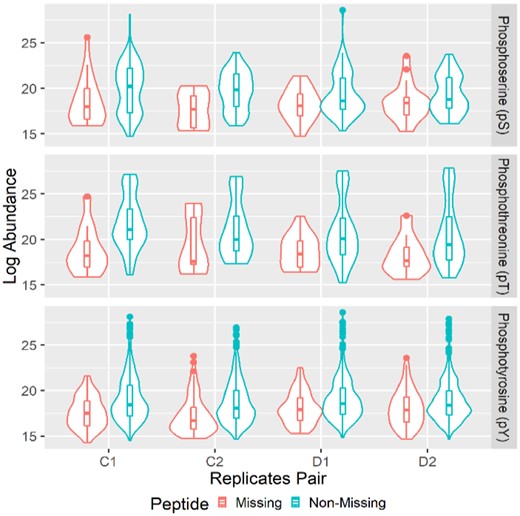
Missing pattern in MS proteomics technical replicates. Each panel shows the log abundance of ‘non-missing’ and ‘missing’ pY, pS or pT per pair of technical replicates by violin and box plots. On the x-axis, C1, C2 represent two biologically control samples, and D1, D2 represent two biologically samples treated by Dasatinib

3.2 Imputation performance—simulated data

To assess the performance of GMSimpute in comparison to other commonly-used methods, an extensive simulation study with 80 scenarios was completed. The complete data matrix was simulated from a MVN distribution, where the mean and covariance used in data generation are derived from the TCGA breast cancer (BC) metabolomics data (N = 30) (Tang et al., 2014). We selected 350 aligned metabolites (or features)-each contained no more than 50% missing values-from this real dataset to compute mean and covariance using the log-abundances. In the simulated complete data matrices, missing values were generated by varying proportions of AIM (and ADM). The distributions of simulated missing and non-missing values were visualized in Supplementary Figure S8. When the AIM proportion is low, the peptides in the missing set have low abundance as simulated. As the proportion of AIM increases (from left to right panel), there are more missing peptides with higher abundance levels. It shares some resemblance to some of the observed patterns in the real datasets in Figure 1.

The imputation performance was evaluated by the compound/peptide-wise Pearson correlation and normalized root mean square errors (NRMSE) between the complete and imputed log abundance for all samples, with NRMSE computed as NRMSE = $\sqrt{{\sum }_{n=1}^N{{(y}_{\mathit{kn}}-{\widehat{y}}_{\mathit{kn}})}^2}/(N\left(\max \left(y_k\right)-\min \left(y_k\right)\right))$⁠. Using the aforementioned missing data generating procedure, each scenario contains only one simulated dataset, since correlation and NRMSE are compound/peptide-wise and there are $M=350$ observations for each metric. Except for the scenario with AIM being small (i.e. 20%) for sample size of N = 30, the TS-Lasso generally outperforms other methods (Supplementary Fig. S9). Therefore, we used TS-Lasso as the default and only set GMSimpute to the compound minimum method for the four scenarios with 80% of missing below LOD when N ≤ 30.

The results show that GMSimpute outperforms other methods, especially when the sample size is large (N > 30). The Pearson correlation presented in Figure 2 and the NRMSE presented in Figure 3 both illustrate that the performance of compound minimum or overall minimum decreases sharply as the AIM proportion $\pi$ increases, and is always worse than the other methods for$\mathrm{ }\pi >0.5$⁠. Additionally, imputation by the overall minimum level results in high NRMSE, especially for the scenario $\pi =0.8$⁠. The machine learning methods of RF, KNN and KNN-TN have higher prediction power than compound or overall minimum for$\mathrm{ }\pi >0.5$⁠, but have poor performance at$\mathrm{ }\pi <0.5$⁠. According to NRMSE, GMSimpute is superior to the remaining methods across all scenarios regardless of the proportion of AIM. Finally, the performance of GMSimpute at N = 120 240 is stable across all scenarios in terms of Pearson correlation and NRMSE, which is not observed in any of the other methods. In the simulated datasets, the DanteR model-based approach (Karpievitch et al., 2009) was not applied, since the metabolite groups and phenotypes were not used for generating the abundance matrix.

Fig. 2.

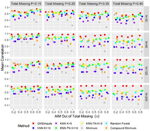
Pearson correlation on simulated abundance. The mean of Pearson correlation between the true and imputed values are presented for each scenario at different sample sizes. For each level of missing percentage, scenarios are ordered by increasing the proportion of AIM from left to right

Fig. 3.

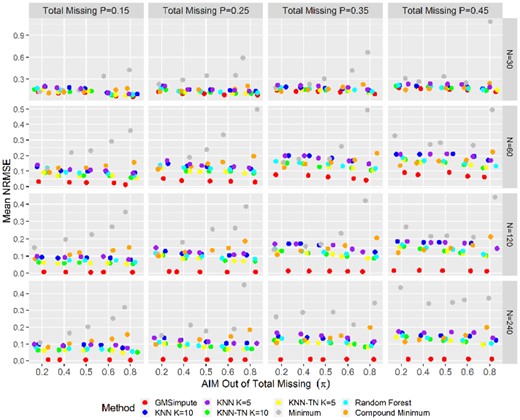
Normalized root mean square errors on simulated abundance. It shows the mean of NRMSE between the true and imputed values across scenarios. For each level of missing percentage, scenarios are ordered by increasing proportion of abundance independent missingness from left to right

3.3 Imputation performance—metabolomics and proteomics data in cancer studies

In addition to the simulated data, two metabolomics datasets and two proteomics datasets in cancer research were also used as the basis for the simulation study. For metabolomics studies, the first dataset contains 25 TCGA BC estrogen receptor (ER) positive or negative samples and five normal breast specimens with 399 known metabolites (Tang et al., 2014). The second is from the TCGA clear cell renal cell carcinoma (ccRCC) study (Hakimi et al., 2016), consisting of 138 matched tumor and normal tissue pairs and 877 identified metabolites, 299 of which are unknown. The first proteomics dataset contained 56 BC ER positive tumor samples from a study in the Netherlands (De Marchi et al., 2016) with ‘Good’ versus ‘Poor’ tamoxifen treatment outcome. The second proteomics dataset contained 31 colon versus 31 rectum adenocarcinoma tumor samples without treatment from TCGA colorectal study (Cancer Genome Atlas Network, 2012).

For TCGA BC metabolomics data, we used all 30 tumor and normal samples and subset to $M=193$ of non-missing metabolites as the complete abundance dataset. In contrast, the tumor samples in the ccRCC metabolomics study were excluded in order to obtain more non-missing metabolites as the complete abundance matrix, i.e. 138 ccRCC normal samples with $M=197$ metabolites. Using these two complete metabolomics datasets, missing abundance values were generated for 60% of the metabolites as described in the aforementioned simulation study. The samples in the BC study were divided into three groups of pronounced difference, i.e. normal, ER positive and ER negative. The clinical groups for the ccRCC study normal samples were grouped by the grade of matched tumor tissue, between which there might not be any biological differences.

We applied DanteR ANOVA model-based imputation method (Karpievitch et al., 2009; Taverner et al., 2012) along with TS-Lasso only to the proteomics datasets, quantified by MaxQuant (Tyanova et al., 2016) but not the metabolomics datasets, since this model-based method was designed to impute proteomics abundance based on the effect of peptide, protein and treatments (Karpievitch et al., 2009). For both proteomics datasets, we randomly selected 1000 peptides without missing values as the complete abundance matrix. Missing patterns were simulated for 60% of the peptides by the same missing value-generating pipeline.

We first evaluated the performance of each method by Pearson Correlation on log abundance for TCGA metabolomics datasets. Figure 4 illustrates that TS-Lasso outperforms the other methods in prediction accuracy, especially for the ccRCC study. For studies with sample size around N = 30, compound minimum outperformed the other methods if at least half of missing values were ADM. On the other hand, TS-Lasso, KNN-TR and RF had similar performance and outperformed the other methods if the random missing proportion was higher than that of missing below LOD. The bar charts in Supplementary Figure S10 displayed the performance of the model-based and TS-Lasso methods on the proteomics data, which confirmed the power of TS-Lasso without using labels of peptides, proteins and study groups in MS/MS study.

Fig. 4.

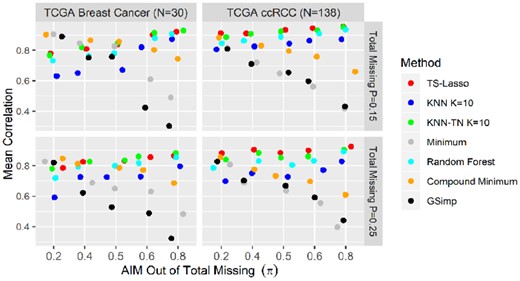
Pearson correlation on TCGA metabolomics studies. The mean of Pearson correlation between the true and imputed values in each TCGA study is presented across scenarios

3.4 Impact on Log2 fold change and differential analysis—TCGA metabolomics data

Based on the Pearson correlation in Figure 4, we further assessed the top five methods for impact on two-group log2 fold change (LFC) of abundance. The LFC in TCGA BC and ccRCC studies was computed between tumor versus normal and high (G3, G4) versus low (G2) grades, respectively. We calculated LFC per metabolite for the imputed matrix and the complete abundance matrix, respectively, and then compared the ratio LFC_imputed/LFC_complete by the boxplots in Figure 5. This ratio is expected to be one for an ideal imputation. A negative ratio indicates that imputation changed the direction of up/downregulation, while a ratio near zero means imputation eliminated (or minimized) the LFC.

Fig. 5.

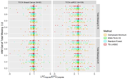
Ratio of LFC between the imputed and complete abundance matrix on TCGA metabolomics data. Ratio >1: LFC enlarged and no change in upregulation; 0<ratio<1: LFC reduced but no change in upregulation; ratio<0: upregulation reversed; ratio=1: no change on LFC

TS-Lasso, KNN-TN, RF and compound minimum did not change the upregulation in the imputed metabolites except for a few outliers in both studies. TS-Lasso and KNN-TN displayed ratio near one, indicating the smallest change in LFC size for the large-scale study, and had similar performance as compound minimum in the small-scale study. Similar results of LFC on the proteomics datasets were presented in Supplementary Figure S11, comparing the same imputation approaches along with DanteR model-based method.

As another way to assess the performance of imputation methods in real data, differential analysis between clinical features in the two TCGA metabolomics studies were as assessed for the complete and imputed abundance matrices. The differential analysis was implemented by Bioconductor R package, limma (Smyth, 2005), on the log-transformed abundances with testing completed by F-test. The imputation methods were first evaluated by Pearson correlation of the log10 adjusted P-values between the complete and imputed matrices similar to the metric in Wei et al., (2018b). Next, we compared the overlap and disagreement of significant features between imputed and complete matrices by area under the receiving operation characteristic curve, true positive rate (TPR) and false positive rate (FPR). The significant metabolites for imputed or complete matrices were selected based on the P-values adjusted by Benjamin–Hochberg false discovery rate (FDR) (Benjamini and Hochberg, 1995) and a threshold of FDR < 5% for BC study and FDR < 10% for ccRCC study. Since GSimp’s performance was comparable to compound minimum, GSimp was not included in differential analysis.

The correlation between the differential analysis log10 adjusted P-values for the ‘pseudo complete’ data and the imputed data are shown in Table 1 and Supplementary Tables S1 and S2. The application of TS-Lasso resulted in the most accurate and stable DE analysis results, especially for the ccRCC large sample size study. KNN-type methods’ performance always depends on the value of K. TS-Lasso had stable and better performance in most scenarios according to the magnitude of impact on differential analysis P-values. The area under the curve, TPR and FPR values for the ‘significant’ biomarkers detected at a threshold of FDR between the complete and each imputed abundance matrix are listed in Supplementary Table S3. The power or TPR for TS-Lasso is always higher than the other methods with type I error or FPR controlled.

Table 1.

Pearson correlation of differential analysis log10 adjusted P-values in between the complete and imputed data for TCGA metabolomics studies, with known metabolites only

Missing (AIM, ADM)	TS-LASSO	Random Forest	KNN-TN (K=5)	Compound minimum
	TCGA breast cancer (N=30)
3%, 12%	0.858	0.780	0.796	0.861
6%, 9%	0.903	0.796	0.836	0.850
7.5%, 7.5%	0.921	0.813	0.851	0.876
9%, 6%	0.927	0.829	0.878	0.812
12%, 3%	0.959	0.899	0.918	0.790
	TCGA ccRCC (N=138)
3%, 12%	0.917	0.908	0.914	0.913
6%, 9%	0.903	0.886	0.893	0.914
7.5%, 7.5%	0.930	0.895	0.919	0.846
9%, 6%	0.955	0.936	0.946	0.861
12%, 3%	0.982	0.967	0.973	0.819

4 Discussion

The simulation study in this paper thoroughly covers a comprehensive collection of missing patterns applied to MS metabolomics data with different sample sizes. Analysis of the real and simulated data found the TS-Lasso method can outperform many commonly-used methods, particularly when the sample size is large (N > 30), because it uses the linear dependencies between metabolites. For downstream differential analyses in application, this imputation method can also identify differentially expressed features with higher accuracy. Interestingly, GMSimpute performance in the real data was less apparent than that in the simulated data, because the abundance of metabolites in simulated data were generated from MVN distribution and the correlation between metabolites was more significant compared to that in the real datasets. A benefit of the TS-Lasso method is that the recovery of undetected peak’s intensity does not require MS profiling information, such as m/z value or retention time. Additionally, the GMSimpute approach selects predictors among all candidate metabolites without restriction on the number of predictors. There are also alternative machine learning tools based on generalized linear regression framework, such as Elastic-Net Generalized Linear Models (Hui and Trevor, 2005) and Support Vector Regression (Basak et al., 2007). However, these methods require specification of parameters that cannot be automatically tuned by the corresponding R packages.

Finally, GMSimpute does not require the specification for the missing data pattern (e.g. specific designation of peaks that are MNAR, MCAR and MAR) and performs consistently well. It is worthwhile to note that GMSimpute allows imputation for metabolites with missing value proportion as much as ∼50%, which is higher than the traditional 20% missing rate, based on the ‘80%’ non-missing value rule (Smilde et al., 2005). On the other hand, the metabolites with more than 50% missing values are still removed in TS-Lasso imputation as the method may not provide accurate prediction if the full matrix is too small. We suggest 40% as the minimum proportion for non-missing metabolites in TS-Lasso imputation in this study. When the non-missing metabolites are low (or lower than 40%), we could perform multi-step-Lasso by first imputing a subset of metabolites via TS-Lasso to increase the proportion of ‘non-missing’ metabolites in all samples. Then, we could use the augmented ‘non-missing’ metabolites to predict the remaining missing abundance via TS-Lasso again.

Future work should focus on improving the performance of GMSimpute in the context ADM or AIM and small sample size. Further investigation is needed to identify metabolites or peptides missing below LOD. Imputation for this pattern should be improved to account for the lower mean abundance and higher proportion of missing. The impact of peptide-specific LOD, co-elution and ion abundance competition on imputation could also be investigated in the future. For small MS studies, re-extracting peaks at targeted range of m/z value and retention time, e.g. MS-DIAL and apLCMS, is a good option to recover missing features. Therefore, future research on imputation for small studies should integrate the peaks or ions information (e.g. adduct, m/z value and retention time for LC-MS).

5 Conclusion

In summary, GMSimpute uses Lasso in a two-step procedure to improve the recovery of all possible types of missing abundance in MS data and provides accurate downstream differential expression analysis, especially in the setting of large sample sizes.

Acknowledgements

We thank Alvaro Monteiro, Jiannong Li, Paul Stewart and Guolin Zhang for the helpful discussion.

Funding

This work by Li was supported in part by Environmental Determinants of Diabetes in the Young (TEDDY) study, funded by the National Institute of Diabetes and Digestive and Kidney Diseases (NIDDK). The work was funded in part by Anna-Valentine Cancer Fund Focused Interactive Group (FIG); and the National Institutes of Health/the National Institute of Child Health and Human Development grant [U54 HD090258] (PI: J. Steven Leeder). This work was also supported by the Biostatistics and Bioinformatics Shared Resource and the Proteomics and Metabolomics Core, funded by the National Cancer Institute as part of Moffitt’s Cancer Center Support Grant [P30-CA076292].

Conflict of Interest: none declared.