DEEPCON: protein contact prediction using dilated convolutional neural networks with dropout

Abstract

Motivation

Exciting new opportunities have arisen to solve the protein contact prediction problem from the progress in neural networks and the availability of a large number of homologous sequences through high-throughput sequencing. In this work, we study how deep convolutional neural networks (ConvNets) may be best designed and developed to solve this long-standing problem.

Results

With publicly available datasets, we designed and trained various ConvNet architectures. We tested several recent deep learning techniques including wide residual networks, dropouts and dilated convolutions. We studied the improvements in the precision of medium-range and long-range contacts, and compared the performance of our best architectures with the ones used in existing state-of-the-art methods. The proposed ConvNet architectures predict contacts with significantly more precision than the architectures used in several state-of-the-art methods. When trained using the DeepCov dataset consisting of 3456 proteins and tested on PSICOV dataset of 150 proteins, our architectures achieve up to 15% higher precision when L/2 long-range contacts are evaluated. Similarly, when trained using the DNCON2 dataset consisting of 1426 proteins and tested on 84 protein domains in the CASP12 dataset, our single network achieves 4.8% higher precision than the ensembled DNCON2 method when top L long-range contacts are evaluated.

Availability and implementation

DEEPCON is available at https://github.com/badriadhikari/DEEPCON/.

1 Introduction

For a protein whose amino acid sequence is obtained using a protein-sequencing device, three-dimensional (3D) models may be predicted using template modeling or ab initio. Template-modeling methods search for other similar protein sequences in a database of sequences whose 3D structures have already been experimentally determined using wet-lab experiments and use them to predict 3D models of the input sequence. The total number of protein structures determined through experimental methods such as X-ray crystallography and Nuclear magnetic resonance spectroscopy are currently limited to 147 817 as of January 2019 (Berman, 2000). Protein sequences for which such templates cannot be found need to be predicted ab initio, i.e. without the use of any structural templates. For structure prediction of protein sequences whose structural templates are not found, predicted protein contacts serve as the driver for folding (Michel et al., 2018; Wang et al., 2017).

Residue-residue contacts or inter-residue contacts (or just contacts) define which pairs of amino acids should be close to each other in the 3D structure, i.e. pairs that are in contact should remain close and those that are not should stay farther. As defined in the Critical Assessment of Protein Structure Prediction (CASP) experiments (Monastyrskyy et al., 2016; Moult et al., 2018), a pair of residues in a protein are defined to be in contact if their carbon beta atoms (carbon alpha for glycine) are closer than 8 Å in the native (experimental) structure. In a true (or a predicted) contact matrix not all contacts are equally important. Local contacts, those with sequence separation less than six residues and short-range contacts (with sequence separation between 6 and 12 residues) are not very useful for building an accurate 3D model. They are required for reconstructing local secondary structures but are not helpful to build folded proteins. However, medium-range contacts, the contact pairs that have sequence separation between 12 and 23 residues, and long-range contacts, the ones separated by at least 24 residues in the protein sequence, are necessary for building accurate models.

All top groups participating in the most recent Critical Assessment of Protein Structure Prediction (CASP) 13 experiment, including DeepMind’s AlphaFold method use contacts (or distance bins) for ab initio protein structure prediction. These contacts can be predicted with relatively high precision for protein sequences that have hundreds to thousands of matches in protein sequence databases such as UNICLUST30 (Mirdita et al., 2017) and Uniref100 (Suzek et al., 2007). The sequence hits obtained, in the form of multiple sequence alignments (MSA) serve as an input to algorithms and machine learning methods to predict contact maps. While the overall goal in protein structure prediction is to predict three-dimensional models (3D information) from protein sequences (1D information), predicted protein contacts serve as the intermediate step (2D information). In the absence of machine learning, contacts are predicted from protein sequence alignments based on the principle that evolutionary pressures place constraints on the sequence evolution over generations (Marks et al., 2011). The predicted contacts from these coevolution-based methods are a key input to machine-learning based methods that generally predict more accurate contacts.

Although Eickholt and Cheng (2012) were the first group to apply deep learning for contact prediction, currently, the most successful contact prediction methods use convolutional neural networks (CNNs) fed with a combination of features generated from multiple sequence alignments and other sequence-derived features. After Jinbo Xu’s group first applied CNNs to predict contacts (Wang et al., 2017), CNNs have been found to be particularly well suited and highly effective for the contact prediction problem, mainly because of their ability to learn cross-channel (cross-feature) information (for example, the relationship between predicted solvent accessibility and predicted secondary structure). In Adhikari et al. (2018), we demonstrate that a single CNN-based network delivers a remarkably better performance compared to a boosted deep belief network. Similarly, in Jones and Kandathil (2018) authors demonstrate that a basic CNN-based method can easily outperform another state-of-the-art meta-method based on basic neural networks. Although the recent progress in contact prediction was initially attributed mostly to coevolutionary features generated using methods such as CCMpred (Seemayer et al., 2014) and FreeContact (Kaján et al., 2014), recent findings (AlQuraishi, 2019; Jones and Kandathil, 2018; Mirabello and Wallner, 2018) suggest that end-to-end training is possible in the near future, where the deep learning algorithm may contribute entirely to the performance and these hand engineered features may be found redundant. Most of the recently successful methods for contact predictions, as demonstrated by the recent CASP results, are available for public use. For instance, methods such as RaptorX (Wang et al., 2017), MetaPSICOV (Jones et al., 2015), DNCON2 (Adhikari et al., 2018), PconsC3 (Michel et al., 2017) and PconsC4 (Michel et al., 2018) are either available as a downloadable tool or a web server. Each of these methods use very different CNN architectures, different sets of input features, and self-curated datasets to train and benchmark their methods.

From the perspective of input and output data format, the protein contact prediction problem is similar to depth prediction from monocular images (Eigen, 2014) in computer vision, i.e. predicting 3D depth from 2D images. In the depth prediction problem, the input is an image of dimensions H × W × C, where H is height, W is width and C is number of input channels, and output is a two-dimensional matrix of size H × W whose values represent the depth intensities. Similarly, in the protein contact prediction problem, the output is a contact probability map (matrix) of size L × L and input is protein features of dimension L × L × N, where L is the length of the protein sequence and N is the number of input channels. Depth prediction usually involves three channels (red, green and blue or hue, saturation and value) while in the latter we have much higher number of features such as 56 or 441 (Jones and Kandathil, 2018). Because of large number of input channels, the overall input volume becomes large, limiting the depth and width of deep learning architectures for training and testing. This also greatly affects the training time and requires high-end GPUs for training. These challenges, imposed by large number of input channels, are also observed in other problems such as plant genotype prediction from hyperspectral images. A protein contact matrix and its input features are symmetrical along the diagonal. Most current methods (including this work) consider both upper and lower triangles (above and below the diagonal line) for training, but for prediction and evaluation, average the confidence scores in the upper and lower triangle.

The protein structure prediction problem has some additional unique characteristics. First, the input features for proteins are not all two dimensional. Input features such as length of a protein sequence are scalar or 0-dimensional (0D). For such input features, we create a channel with the same value throughout the channel. Similarly, input features such as secondary structure predictions are one-dimensional (1D) and we create two channels for each 1D input feature of length L—first channel by copying the vector L times to create a L × L matrix, and second channel by transposing the input feature vector and then copying L times to create a L × L matrix. Another way to generate 2D matrix from 1D vector is to compute outer product of the vector with its own transpose. Other input features which are 2D, are copied into the input volume, as they are. Also, the length of a protein sequence can vary from a few residues to a few thousand residues, implying a variable input feature volume. The dimension of each 2D feature (transformed into channels) will depend on the length of the protein. Unlike real-world images, these input features, cannot be easily studied/understood visually towards understanding what the networks are learning. The training and test dataset that we can use is also limited. Unlike other publicly available datasets, the protein structure dataset size cannot be significantly increased because only up to around 11 thousand new structures are experimentally determined each year. What further reduces this dataset is the similarity between many of the structures deposited. On these proteins, if we perform some basic redundancy reductions such as keeping only the proteins with more than 20% sequence similarity and those with high resolution structures, the number of proteins available for training reduces to only around a five thousand (Wang and Dunbrack, 2003). Despite the fact that the data appears to be limited compared to many other datasets, some argue that it is sufficient to capture the principles of protein folding. In addition, a typical protein contact map, which is a binary matrix, is around 95% zeros and 5% ones (Jones et al., 2015).

The three-dimensional models of real-world objects and protein structures have a fundamental difference. Protein 3D models are not scalable. An object, such as a chair, in the real world may be tiny or large. Proteins can also be large or small but the size of structure patterns are always physically fixed. For instance, the size of an alpha helix (a common building block of many protein structures) is the same for proteins of any size. The distance between carbon-alpha atoms is a fixed physical distance whether the helices are in a small helical protein such as the mouse C-MYB protein or a large helical protein such as hemoglobin. Because of this unique characteristic of protein structures, it is yet to be fully understood how useful deep architectures such as U-Nets (Ronneberger et al., 2015) can be for protein contact prediction although some groups have developed contact prediction methods using such architectures (Michel et al., 2018). Similar to the problem of depth prediction, the ultimate goal in the field is to develop methods that can be scaled to predict physical distances map (in Angstroms). Since raw distance prediction is too difficult, some groups have developed methods that can predict contacts at various sequence separation thresholds (Xu, 2018) and demonstrate that such binning of distance ranges improves contact prediction at a single standard distance threshold, such as the standard of 8 Å.

In this work, we demonstrate that dilated residual networks with dropout layers are best suited for addressing the protein contact prediction problem. It can be argued that the results in a small dataset may not hold true in large datasets. In addition, results generated using one kind of features may not hold true for another kinds of input features. For instance, methods that work well for sequence-based features (such as secondary structures) may not work well for features generated directly from multiple-sequence alignments (such as covariance matrix and precision matrix). When trained on the DeepCov dataset consisting of 3456 proteins, using the same dataset and input features for training, our method achieves up to 6 and 15% higher precision on the PSICOV150 protein dataset (independent test set) when top L/5 and L/2 long-range contacts are evaluated, respectively (L is protein length). Similarly, when trained on the DNCON2 dataset consisting of 1426 proteins, using the same dataset for training and testing, a single network in our method achieves 4.8% higher long-range precision (top L). While DNCON2 uses a two-level approach combined with ensembling of 20 models, we use a single network. Although we trim the input length of a protein to 256 for all proteins in our training experiments, after the training, our models can make predictions for a protein of any length. It is important to note that although our overall architecture is novel, we are not the first group to apply dilated residual networks for protein contact prediction. In the CASP13 meeting, DeepMind’s group were the first group to present that dilated convolutional layers are fit for this problem.

2 Materials and methods

2.1 Datasets

For training our models in our experiments, we use two datasets: (i) the DNCON2 dataset (Adhikari et al., 2018) available at http://sysbio.rnet.missouri.edu/dncon2/ and (ii) DeepCov dataset (Jones and Kandathil, 2018) available at https://github.com/psipred/DeepCov. Following the deep learning practice, for each experiment, we consider three subsets—training subset, validation subset and an independent test set. The DNCON2 dataset consists of 1426 proteins between 30 and 300 residues in length. The dataset was curated before the CASP10 experiment in 2012 and the protein structures in the dataset are of 0 to 2 Å in resolution. These proteins are filtered by 30% sequence identity to remove redundancy. Of the full dataset, we use 1230 proteins for training and the remaining 196 as the validation set. We found that the protein with PDB ID 2PNE in the validation set was skipped during evaluation in the DNCON2 method and hence we too skip it. We train and validate our method using the 1426 proteins and test on 62 protein targets in the CASP12 experiment. The CASP12 protein targets range from 75 to 670 residues in length. For evaluating our method on the CASP12 dataset, we predict contacts for the whole protein target and evaluate the contacts on the full target (or domains). The DeepCov dataset consists of 3456 proteins used to train and validate models, i.e. tune hyperparameters. The models trained using the DeepCov dataset are tested on the independent PSICOV dataset consisting of 150 proteins.

2.2 Contact evaluation

Following the standard in the field (Monastyrskyy et al., 2016), as evaluation metrics of contact prediction accuracy, we use the precision of top L/5 predicted long-range contacts (P_L/5-LR), where L is the length of the protein sequence. In addition, we also evaluate our methods using the precision of top L/2 long-range contacts (P_L/2-LR), precision of top L long-range contacts (P_L-LR) and the precision of all medium- and long-range contacts (P_NC-MLR). To calculate P_NC-MLR for a protein with NC number of medium- and long-range contacts, we first round top NC medium- and long-range predicted probabilities (after ranking the probabilities) to 1 s and the rest to 0 s. Precision is then calculated as the ratio of ‘the number of matches between predicted and true matrix’ and NC.

2.3 Input features

We use two kinds of features in our experiments—covariance features (as in the DeepCov method), and sequence features generated using various prediction methods (as in the DNCON2 method). The sequence features consist of eight groups of features as input for training and validating our models. These include scalar values such as sequence length, one-dimensional features such as solvent accessibility and secondary structure predictions, and two-dimensional features such as features computed from position specific scoring matrix, sequence separation information, pre-computed statistical potentials, features computed from input multiple sequence alignment, and coevolution predictions from the alignment. In total, we use 29 unique features as input which we roll out to 56 input channels in total. For each 0D (scalar) feature we copy the value into the entire channel. Similarly, we copy each 2D input feature as-is into the final input volume as a single channel. For each 1D input feature for a protein of length L, we create two channels—first channel by copying the vector L times to create a L × L matrix, and second channel by transposing the input feature vector and then copying L times to create an L × L matrix. Although the maximum length of a protein in this dataset is 300, we trim all input features to 256 length so that the longest protein has an input volume of 256 × 256 × 56. For training, all proteins with length less than 256 are 0-padded so that all input volumes have the same dimension of 256 × 256 × 56. The covariance feature consist of a 441 channel covariance matrix calculated using the publicly available script (cov21stat) and dataset in the DeepCov package. For this dataset the input volume for each protein is L × L × 441. For generating multiple sequence alignments for the CASP dataset and the DNCON2 dataset, we follow the approach of using HHsearch (Söding, 2005) with the UniProt20 database (2016/02 release) followed by JackHmmer (Finn et al., 2011) with the UniRef90 database (2016 release) as discussed in the DNCON2 method (see our DNCON2 paper for details). These databases are publicly available at http://sysbio.rnet.missouri.edu/bdm_download/dncon2-tool/databases/. The alignments for the proteins in the DeepCov dataset and the PSICOV150 dataset were copied from the corresponding DeepCov repository.

2.4 Training convolutional neural networks

Our ConvNets involve an input layer, a number of 2D convolutional layers with batch normalization or dropouts, residual connections and Rectified Linear Units (ReLU) activations. In all architectures, the final layer is a convolutional layer with one filter of size 3 × 3 followed by a ‘sigmoid’ activation to predict contact probabilities. Besides dropout no other regularizes (such as L2) were used and ADAM (Kingma and Ba, 2014) was used as the optimizer. Since we only have convolutional layers, the variables are the numbers and size of filters at each layer, and dilation rate when dilated convolutional layers are used. Figure 1 summarizes our approach. All the CNN filters in the first layer convolve through the input volume of 256 × 256 × N producing batch normalized and ‘relu’ activated outputs passed as input to the subsequent layers. The number of channels, N, is 56 when DNCON2 dataset is used and 441 when DeepCov dataset is used. Error is computed using binary cross entropy calculated as −(y log(p)+(1−y) log(1−p)), where p is the output of the sigmoid activation of the last layer for each residue pair, and y is 1 if the residue pair are in contact in the experimental structure or else is 0.

Fig. 1.

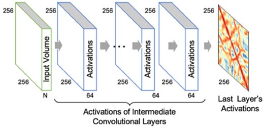
General architecture for training and testing. Filters in the first layer of convolutional neural network slide through the input volume for each protein with a 300 × 300 × 56 matrix (56 input channels) producing activation volumes. One filter in the last layer slides through the activation volume of the previous layer to generate the final activations at each position of the 256 × 256 matrix

Although we crop the input length of our training proteins to 256, after the training the model can make predictions for a protein of any length. Since we do not use max pooling or any dense connections, a model of any arbitrary dimension can be built for predicting proteins of lengths longer than 256 residues. For instance, to predict contacts for a protein of length 500 (i.e. input volume of 500 × 500 × 56), we first build a model of the same input dimensions (i.e. 500 × 500) and then load all the trained weights into this new model and make predictions for the input volume. Since contact matrix is symmetrical, we average the prediction of either triangle to generate final predictions. No model ensembling techniques were used. In all our training experiments, we reduce the learning rate by 0.5 when the loss on the validation dataset does not improve for 10 epochs. We stop the training if the loss on the validation dataset does not improve for 20 epochs in a row, and the output at the last epoch is selected.

We used the Keras library (https://keras.io/) with Tensorflow (Abadi et al., 2016) backend for our method development. On a machine with 2 CPUs and 24 GB memory with a NVIDIA Tesla K80 GPU the training (around 35–45 epochs) takes about 16 h for either of the DNCON2 or DeepCov dataset. For testing larger architectures we used the Tesla P100, V100 and Quadro P6000 GPUs.

2.5 Network architectures

We start our training experiments with standard convolutional neural networks (or fully convolutional networks), each preceded by a batch normalization layer and ReLU activation. We find that performance of such networks drop after 32–64 convolutional layers. Next, we design a residual block consisting of two convolutional layers, each preceded by a batch normalization layer and ReLU activation. Fixing the total number of convolutional filters in each layer to 64, we design four residual networks: (i) a regular residual network with depths (number of blocks) as the key parameter, (ii) an architecture with the second batch normalization layer in each residual block replaced with a dropout layer, (iii) we replace the last convolutional layer with a dilated convolutional layer with dilation rate alternating among 1, 2 and 4 and (iv) an architecture that is a combination of the second and third architecture, i.e. we replace the second batch normalization layer with a dropout layer, and replace the second convolutional layer with a dilated convolution layer at alternating dilation rates of 1, 2 and 4 (see Fig. 2). We also tested many other architecture variations such as filter sizes of 16, 24 and 32, and different ways to alternate between batch normalization layers and dropout layers. On average, these architectures were not significantly better than the four architectures we discuss above.

Fig. 2.

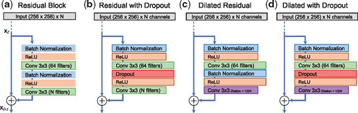
Residual network architectures designed for training and evaluation. (a) Standard residual block, (b) Standard residual block with second batch normalization layer replaced by a dropout layer, (c) Standard residual block with second convolution layer replaced with dilated convolutions, and (d) Standard residual block with dropout and dilation

Using the DNCON2 dataset as our training and validation set and CASP12 targets as test dataset, we compared the precision of a fully convolutional network (FCN), and the four residual architectures—standard residual network, residual network with dilation, residual network with dropout and residual network with dilation and dropout. On the fully convolutional networks and residual networks, we experimented adding dropout layers in many ways and found that alternating between batch normalization layers and dropout layers yield the best performance (Zagoruyko and Komodakis, 2016). On our standard residual network with 64 layers having 64 3 × 3 filters in each layer, we tested dropout values of 0.2, 0.3, 0.4 and 0.5. When we evaluated these models using the precision of top L/5 long-range precision (P_L/5-LR) and all medium-, and long-range precision (P_NC-MLR) we found that specific value of dropout does not matter as long as we have the dropout layers in place. For most of our experiments we fixed 0.3 as the parameter for our dropout layers (i.e. keep 70% weights).

Since our findings resonate with the findings in Zagoruyko and Komodakis (2016) we also hypothesize that the issue of ‘diminishing feature reuse’ is pronounced in the problem of contact prediction and that the dropout layers partially overcome the issue. In fact, we observed up to 6% gain in P_L/5-LR when we randomly replace some of the initial batch normalization layers in a fully convolutional layers with just 16 layers (each having 64 filters). These findings suggest that dropout layers, when used appropriately, can be highly effective in network architectures for protein contact prediction. When evaluated on the independent CASP12 dataset consisting of 62 targets, we find that residual networks with dilation and dropout outperform all the four other architectures, across all the precision metrics, P_L/5-LR, P_L/2-LR, P_L-LR and P_NC-MLR (see Fig. 3). We call this residual network with dilation and dropout as the DEEPCON method.

Fig. 3.

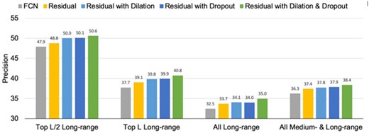
Comparison of the precision on CASP12 dataset obtained from various architectures when models are trained and validated using the DNCON2 dataset

3 Results

3.1 Comparison of network architectures with other network architectures

To benchmark our DEEPCON architecture we compared it with the architectures used in the current state-of-the-art methods—Raptor-X (Wang et al., 2017), DNCON2 (Adhikari et al., 2018), DeepCov (Jones and Kandathil, 2018) and PconsC4 (Michel et al., 2018). The Raptor-X method uses residual networks with around 60 convolutional layers. The DNCON2 method uses ensembled two-level convolutional neural network, each with 7 layers. Each network consists of six layers with 16 filters each and an additional convolutional layer with one filter for generating the final contact probabilities. Each convolutional network here has around 50 thousand parameters. In the DeepCov method, 441 input channels are reduced to 64 using a Maxout layer, and then fully convolutional layers of various depths are tested. DeepCov performs best at the receptive field size of 15, i.e. 7 convolutional layers. The PconsC4 method directly uses the U-Net architecture that accepts 256 × 256 × 64 input volume, i.e. input channels will be first projected to 64 channels. Such an architecture has 31 million parameters.

Using covariance matrix as the input feature, when we use DeepCov dataset for training and validation and PSICOV 150 proteins as the test dataset, we find that DEEPCON performs similar to the standard residual architecture (see Fig. 4) on P_L/5-LR evaluation metic. On the P_NC-LR and P_NC-MLR metrics, however, DEEPCON’s performance is significantly higher than the standard residual-type network architecture, a fully connected CNN architecture, and the U-Net architecture. Similarly, using sequence features as input, when we use DNCON2 dataset for training and CASP12 protein domains for testing, we observe similar results (see Fig. 4). DEEPCON architecture’s high performance on these two very different datasets suggests that deep residual networks with dropout are reliable and work well for a variety of input features towards predicting protein contacts.

Fig. 4.

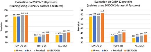
Comparison of the performance of various ConvNet architectures—fully connected ConvNets (FCN), residual networks with dropout and dilation (DEEPCON), regular residual network and U-Net like architecture—using P_L/5-LR, P_L-LR and P_NC-MLR. We train and validate using the DeepCov dataset consisting of 3456 proteins and test (the results here on left) using the PSICOV 150 dataset using the covariance features (left). We train and validate using the DNCON2 dataset consisting of 1426 proteins and test using the 62 proteins in the CASP12 dataset (the results on the right) using the sequence features (right)

3.2 Performance of DEEPCON

We compared the performance of our method DEEPCON with two state-of-the-art methods that have their training dataset publicly available. First, we compared the performance of DEEPCON with the DeepCov method when trained and tested using the same dataset consisting of 3456 proteins. Using the covariance features as input and with the first 130 proteins as the validation set (as done in DeepCov) we train our models and test them on the independent PSICOV dataset consisting of 150 proteins. Evaluating our predictions on the PSICOV150 dataset, we find that our implementation performs better than the DeepCov method when we develop an architecture that is similar to the one used in the DeepCov method (see Table 1). Next, we compare DEEPCON’s performance with DeepCov method using P_L/5-LR and P_L-LR. Our comparison (see Table 1) shows that DEEPCON achieves 5.9% improvement in P_L/5-LR and 15% improvement in P_L-LR. For a fair comparison we only train our models once on the DeepCov dataset. In fact, to reduce our training time (and because of resource limitations), we trim all proteins to 256 residues length, possibly using lesser input information than the information used by the DeepCov method.

Table 1.

Comparison of DEEPCON’s performance with DeepCov and DNCON2

Training and validation dataset	Test dataset	Features used	Architecture	PL/5-LR	PL-LR
DeepCov dataset (3456 proteins)	PSICOV (150 proteins)	Covariance Matrix	DeepCov (Jones and Kandathil, 2018)	85.8	55.1
			DeepCov like (our implementation)	88.6	58.2
			DEEPCON	90.9	63.4
		Sequence Features	DEEPCON	92.6	68.2
DNCON2 dataset (1426 proteins)	CASP12 (84 domains)	Covariance Matrix	DEEPCON	55.9	36.3
		Sequence Features	DNCON2 (Adhikari et al., 2018)	59.9	39.1
			DEEPCON	61.5	41.0

Next, using sequence features as input, we compared DEEPCON’s performance with the DNCON2 method when trained and tested on the 1426 proteins dataset that was used to train DNCON2. While DNCON2 uses two-level approach exploiting information from distance thresholds other than the standard 8 Å and use model ensembling, we train a single model. For training our models we use the same set of 196 proteins as validation set and the remaining as the training set (as done in the DNCON2 work) and evaluate on the CASP12 dataset consisting of 84 domains. For all our predictions, we use the exact same input features (generated for targets instead of domains) as used by DNCON2. On these 84 CASP12 domains, we find that DEEPCON achieves 3.2% higher P_L/2-LR and 4.8% higher P_L-LR (see Table 1). For completeness, in Table 1, we also report the performance of our DEEPCON architecture when it is trained and validated on the DeepCov dataset with sequence features as input and on the DNCON2 dataset with covariance features as input.

Furthermore, to verify that the improved contact predictions are indeed useful, for the 150 proteins in the PSICOV dataset, we predicted full three-dimensional (3D) models using CONFOLD2 (Adhikari and Cheng, 2018). CONFOLD2 is ideal here because it purely relies on the input predicted contacts information to build models, unlike methods that use template fragments. It iteratively selects top 0.1 L, 0.2 L, 0.3 L, etc., up to 4.0 L input contacts, generates up to 200 decoys and automatically selects top five models. For the PSICOV dataset, using the covariance features as input, we predicted contacts using the DeepCov method and our DEEPCON method, and filtered the contacts to keep only the medium-range and long-range contacts. These contacts were supplied as input to CONFOLD2 to obtain full-atom 3D models. Next, we evaluated the top-five models predicted by CONFOLD2 and compared the best-of-top-five. Comparison of the predicted contacts using P_L-LR and the best models using TM-score (Zhang, 2005) shows that, on average, DEEPCON contact predictions are better than DeepCov contacts (see Fig. 5). From the same figure, we also infer that the improvement in DEEPCON is not limited to proteins for which large number of homologous sequences are found. We calculated effective homologous sequences (Neff) using the ‘colstats’ program in the MetaPSICOV package. Finally, following the practice to evaluate the calibration of predicted contacts (Liu et al., 2018; Jones and Kandathil, 2018; Monastyrskyy et al., 2016) (i.e. to check if our probabilities are underestimated or overestimated), we evaluated the precision of contacts predicted at various confidence intervals and found that DEEPCON’s probabilities are highly calibrated (see Fig. 6).

Fig. 5.

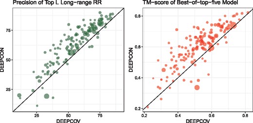
Comparison of the contacts predicted by the DeepCov method and our DEEPCON method on the PSICOV150 dataset using P_L-LR (left) and the best-of-top-five models predicted by CONFOLD2 (right) using TM-score. The average TM-score of the best-of-top-five models by DEEPCON and DeepCov are 0.60 and 0.52 respectively. The size of the points in the plot correspond to the relative difference in the effective number of sequences (Neff) in the input alignment file, i.e. smaller points represent proteins with small Neff. The Neff values range from 14 to 25 702

Fig. 6.

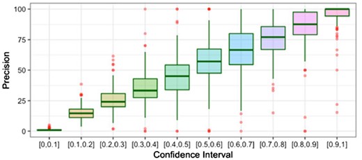
Boxplot of precision of DEEPCON contacts at various confidence intervals, predicted for the PSICOV150 dataset

We believe that there are three reasons for DEEPCON’s improved performance. In Table 1 we show that when DEEPCON’s architecture is scaled back to an architecture similar to the DeepCov method’s architecture, the improvement is still significant. This suggests that the overall training and testing parameters (such as optimizer) and the overall training framework built using Tensorflow and Keras is contributing to the improvement. DEEPCON’s deeper architecture consisting of 32 residual blocks (effectively 64 convolutional layers) and the use of Dropout and BatchNormalization in the residual block, as shown in Figure 3, are also contributing to the improvement.

3.3 Evaluation on CASP 13 dataset

Finally, we compare our DEEPCON method trained using the covariance features from the DeepCov dataset with a few state-of-the-art methods that accept multiple sequence alignment as input. For this comparison, we consider the 20 proteins targets (consisting of 32 domains) in the CASP 13 dataset for which the native structures are publicly available. Although it would be ideal to evaluate on the entire CASP 13 dataset, as done by the CASP assessors, we are only able to evaluate the targets whose native structures are available to us. These 20 protein targets include both free-modeling (FM) and template-based modeling (TBM) domains. First we predicted multiple sequence alignments for these 20 protein targets using the publicly available DNCON2 scripts to generate multiple sequence alignments. As done in the DNCON2 method, we use the sequence databases curated in 2012. Next, we predicted contacts using the DEEPCON method we developed, and evaluated the contacts on the 32 domains. We also downloaded the PconsC4 tool available at https://github.com/ElofssonLab/PconsC4/ and predicted contacts. Similarly, we also downloaded the DeepCov method available at https://github.com/psipred/DeepCov and predicted contacts with the same alignment files as input. To obtain a baseline we also predicted contacts using CCMpred and FreeContact. To obtain reference results, we evaluated the contact predictions of the top group in CASP13 over these 20 targets, and also submitted the alignments to the Raptor-X webserver at http://raptorx.uchicago.edu/ContactMap/ and evaluated the contacts predicted by the webserver. We use the same alignment file as input to all these methods.

Table 2 shows that our method DEEPCON performs better than the baseline methods CCMpred and FreeContact, and better then PconsC4 and DeepCov. Our comparison of DEEPCON, DeepCov and PconsC4 with the RaptorX web-server is only for a reference because it uses many additional features other than the covariance calculated from raw alignment files. It is worth noting that the top group in CASP13 experiment was the RaptorX method. The large difference between the top group’s performance in CASP13 and the performance of the RaptorX webserver with our alignments as input (in Table 2), and the fact that the RaptorX method used in the CASP13 experiment is not significantly updated from the published method (as mentioned by Dr. Xu in his presentation) highlights the performance gain that could be achieved with better/larger multiple sequence alignments. To further validate our assumption, we also reached out to the top performing groups in the CASP13 experiment asking for their alignment files but we did not receive such data for these 20 targets from the groups. The differences of precision between the baseline methods (CCMpred and FreeContact) and the deep learning methods (DEEPCON, DeepCov and PconsC4) represent the gain from the use of deep neural networks.

Table 2.

Comparison of DEEPCON’s performance with other methods that accept multiple sequence alignment as input on the 32 domains in the CASP13 dataset of 20 protein targets

	PL/5-LR	PL-LR	PL/5-MLR	PL-MLR
* Best Group in CASP13 (RaptorX)	79.6	55.2	88.8	66.5
* RaptorX Webserver	67.4	43.8	75.3	53.2
DEEPCON (our method)	57.2	34.2	67.5	45.9
DeepCov (Jones and Kandathil, 2018)	48.2	28.3	61.6	37.9
PconsC4 (Michel et al., 2018)	42.7	27.3	53.1	34.9
CCMpred (Seemayer et al., 2014)	32.8	19.3	34.8	22.6
FreeContact (Kaján et al., 2014)	30.3	17.4	33.5	20.0

Note: Methods with an asterisk (*) are listed for reference. All methods except for the first (in the first row) use the same alignment file as input.

4 Conclusions

We found that regularization using dropout is highly effective in all architectures—fully convolutional, residual, or dilated residual networks. We also found that dilated convolutional methods yield negligibly better performance than the regular residual networks, but these gains are amplified when dilated convolutions are combined with dropouts. We believe that our findings when combined with techniques such as using multiple distance thresholds (Adhikari et al., 2018; Jones et al., 2015; Michel et al., 2018), ensembling (Adhikari et al., 2018; Wang et al., 2017), predicting actual distances using binning (Xu, 2018), etc. used in other methods can significantly improve the overall contact prediction precision. We also believe that our findings and the architectures will be utilized by other researchers to continue the development and obtain better performance with more complex and powerful architectures, larger training and validation datasets, development of additional features and output labels, and through model ensembling.

Acknowledgements

Some of the computation for this work was performed on the high-performance computing infrastructure provided by Research Computing Support Services (RCSS) and in part by the National Science Foundation under grant number CNS-1429294 at the University of Missouri, Columbia MO. We would like to thank the RCSS team for their infrastructure and technical support. We also thank Google Cloud for cloud credits through the GCP cloud credits program. We also gratefully acknowledge the support of NVIDIA Corporation with the donation of the Quadro P6000 GPU used for this some of the computations in this research. We are also thankful to Cynthia Jobe at the University of Missouri-St. Louis (UMSL) for her review comments, and Chase Richards at UMSL for packaging DEEPCON as a Python library.

Funding

The work was partially supported by the New Faculty Start-up Grant at University of Missouri-St. Louis (UMSL) to BA, and the 2018 UMSL Research Award to BA.

Conflict of Interest: none declared.