P-value evaluation, variability index and biomarker categorization for adaptively weighted Fisher’s meta-analysis method in omics applications

Abstract

Motivation

Meta-analysis methods have been widely used to combine results from multiple clinical or genomic studies to increase statistical powers and ensure robust and accurate conclusions. The adaptively weighted Fisher’s method (AW-Fisher), initially developed for omics applications but applicable for general meta-analysis, is an effective approach to combine P-values from K independent studies and to provide better biological interpretability by characterizing which studies contribute to the meta-analysis. Currently, AW-Fisher suffers from the lack of fast P-value computation and variability estimate of AW weights. When the number of studies K is large, the 3^K − 1 possible differential expression pattern categories generated by AW-Fisher can become intractable. In this paper, we develop an importance sampling scheme with spline interpolation to increase the accuracy and speed of the P-value calculation. We also apply bootstrapping to construct a variability index for the AW-Fisher weight estimator and a co-membership matrix to categorize (cluster) differentially expressed genes based on their meta-patterns for intuitive biological investigations.

Results

The superior performance of the proposed methods is shown in simulations as well as two real omics meta-analysis applications to demonstrate its insightful biological findings.

Availability and implementation

An R package AWFisher (calling C++) is available at Bioconductor and GitHub (https://github.com/Caleb-Huo/AWFisher), and all datasets and programing codes for this paper are available in the Supplementary Material.

Supplementary information

Supplementary data are available at Bioinformatics online.

1 Introduction

High-throughput biological experiments play a key role in deciphering biological mechanisms behind complex diseases. Advanced experimental techniques allow us to obtain high-resolution genomic information with affordable price. Over the years large amount of omics data are accumulated in public databases and repositories: The Cancer Genome Atlas (TCGA) http://cancergenome.nih.gov, Gene Expression Omnibus (GEO) http://www.ncbi.nlm.nih.gov/geo/ and Sequence Read Archive (SRA) http://www.ncbi.nlm.nih.gov/sra/, just to name a few. For a given transcriptomic study from microarray or RNA-seq, many statistical methods have been developed for detecting differentially expressed (DE) genes as candidate biomarkers (Pan, 2002; Soneson and Delorenzi, 2013). The analysis of a single study, however, contains small to moderate sample size (usually N = 20 ∼ 50), producing unstable and inaccurate results (Domany, 2014; Simon, 2005). Meta-analysis to combine multiple transcriptomic studies has become a common practice to improve statistical power and reproducibility. Readers who are interested may refer to Ramasamy et al. (2008) for a practical guideline of microarray meta-analysis, and Tseng et al. (2012); Begum et al. (2012) for comprehensive reviews of microarray and genome-wide association study meta-analysis.

Among the numerous meta-analysis methods proposed in the literature, combining P-values from multiple studies is a simple and flexible solution to combine studies of different experimental design and avoid complexity from batch effect (i.e. systematic non-biological differences between studies because of differences such as sample platforms and experimental protocols; Luo et al., 2010). When combining two studies, it has been demonstrated that such batch effects often cannot be properly removed when by normalization (Guerra and Goldstein, 2009). Meta-analysis methods (e.g. P-value combination methods) will lead to increased statistical power by combining the summary statistics (i.e. P-values). These summary statistics, representing the strength of association, are usually considered standardized and independent of the batch effect (Gibbons et al., 2018). Under the framework of such P-value combination methods, multiple hypothesis testing settings have been considered to address different biological questions. Following the convention of Song and Tseng (2014) (also see Birnbaum, 1954; Li and Tseng, 2011), three major hypothesis settings have been considered in the literature: HS_A targets on the hypothesis testing setting to detect biomarkers that are DE in all cohorts:

$$\begin{array}{c}{H}_0:{\displaystyle \overrightarrow{\theta }}\in \cap \{{\mathrm{\theta }}_k=0\}\\ H_A:{\displaystyle \overrightarrow{\theta }}\in \cap \{{\mathrm{\theta }}_k\ne 0\},\end{array}$$

where HS_A is the acronym for ‘Hypothesis Setting All’ mentioned above, and θ_k is the effect size of study k,$1\le k\le K$⁠). HS_B targets on biomarkers DE in one or more studies:

$$\begin{array}{c}{H}_0:{\displaystyle \overrightarrow{\theta }}\in \cap \{{\mathrm{\theta }}_k=0\}\\ H_A:{\displaystyle \overrightarrow{\theta }}\in \cup \{{\mathrm{\theta }}_k\ne 0\},\end{array}$$

where ‘B’ in HS_B is the counterpart of ‘A’ in HS_A. The HS_B method is traditionally also referred to as ‘union–intersection test (UIT)’ or ‘conjunction null hypothesis’ in the statistical literature. HS_r targets on biomarkers DE in at least r studies:

$$\begin{array}{c}{H}_0:{\displaystyle \overrightarrow{\theta }}\in \cap \{{\mathrm{\theta }}_k=0\}\\ H_A:\sum \mathbb{I}\{{\mathrm{\theta }}_k\ne 0\}\ge r,\end{array}$$

where r in HS_r represents the rth order statistics (Song and Tseng, 2014), $\mathbb{I}\{·\}$ is an indicator function taking value one if the statement is true and zero otherwise, and r is usually pre-specified with$K/2\le r\le K$⁠).

Biologically HS_A is preferred when the purpose is to find concordant genes across all studies. HS_r can be considered as a robust form of HS_A to seek for concordant genes in majority of studies. HS_B is considered when heterogeneity is expected and we are interested in biomarkers statistically significant in at least one study.

In the literature, HS_B is an UIT (Roy, 1953) and is also called a conjunction or intersection hypothesis (Benjamini and Heller, 2008). Many statistical tests have been developed for this hypothesis setting, including Fisher’s method (Fisher, 1992), Stouffer’s (Stouffer et al., 1949) method, the minimum P-value method (also referred as Tippett’s method) (Tippett, 1931) and many others. Fisher’s method defines the test statistic as the sum of log-transformed P-values:$\mathrm{ }{T}^F=-2{\sum }_{k=1}^K\log p_k$⁠, where p_k is the P-value from the kth study; Stouffer’s method uses $T^S=-\frac{1}{\sqrt{K}}{\sum }_{k=1}^K{\mathrm{\Phi }}^{-1}\left(p_k\right)$⁠, where ${\mathrm{\Phi }}^{-1}(·)$ is the inverse cumulative distribution function (CDF) of standard normal distribution. A larger Fisher (or Stouffer) score indicates stronger differential expression evidence. Under the null assumption and assuming independence across studies, the null distribution of Fisher’s statistics follows ${{\chi }^2}_{2K}$ and Stouffer’s follows N(0, 1). Although Fisher’s method has many theoretical advantages (e.g. asymptotic Bahadur optimality under certain restricted Gaussian assumptions; see Littell and Folks, 1971), it has a critical pitfall when heterogeneity is expected across studies. For example, suppose ${{\displaystyle \overrightarrow{p}}}_1=(0.001, 1, 1)$ represents P-values of three studies of Gene 1 and ${{\displaystyle \overrightarrow{p}}}_2=(0.1, 0.1, 0.1)$ represents P-values of Gene 2. Both genes produce the same Fisher’s test statistics and meta-analysis P-values (⁠$T^F=13.8$ and$\mathrm{ }{p}^F=0.032$⁠) but the biological interpretation of the two genes are obviously different. ${{\displaystyle \overrightarrow{p}}}_1$ indicates strong statistical significance only in the first study, while ${{\displaystyle \overrightarrow{p}}}_2$ shows marginal statistical significance in all three studies. To characterize study heterogeneity in meta-analysis, Li and Tseng (2011) proposed an adaptively weighted Fisher’s method (AW-Fisher) where the Fisher’s score is modified as weighted sum and the 0–1 weights can be viewed as latent variables of whether a study contributes DE information to the meta-analysis (details see next paragraph). Aside from additional biological interpretability of AW weights, AW-Fisher also enjoys nice theoretical properties. It has been shown to be admissible (Li and Tseng, 2011) and asymptotic Bahadur optimal under certain Gaussian assumptions (Fang et al., 2019). In addition, Fisher’s method is more powerful when all studies are significant and the minimum P-value method is more powerful when only one study has small P-value. AW-Fisher theoretically takes advantage of both methods on their favored extreme situations (Li and Tseng, 2011). Chang et al. (2013) performed a comprehensive comparative study to evaluate 12 popular microarray meta-analysis methods and categorized them into the three complementary hypothesis settings, ${\text{HS}}_A,\hspace{0.33em}{\text{HS}}_B$ and HS_r. AW-Fisher was the best performer in the HS_B setting when considering a variety of data and heterogeneity assumptions.

Below we describe the method and rationale for AW-Fisher (Li and Tseng, 2011).

For the convenience of discussion, we focus on two class comparison for detecting DE genes in this paper. However, users can easily extend to multi-class, continuous or survival outcomes using conventional packages for differential expression analysis to generate P-values as input of our method. Throughout the manuscript, we use limma (Smyth, 2005) for continuous data (e.g. microarray or RNA-seq RPKM data) and edgeR (Robinson et al., 2010) for count data (e.g. RNA-seq count data) to calculate P-values for each individual study. Define$T({\displaystyle \overrightarrow{\mathbf{P}}};{\displaystyle \overrightarrow{\mathbf{w}}})=-2{\sum }_{k=1}^K{w}_k\mathrm{l}\mathrm{og}{P}_k$⁠, where ${\displaystyle \overrightarrow{\mathbf{w}}}=(w_1,\dots ,w_K)\in {\{0, 1\}}^K$ is the AW weight associated with K studies and ${\displaystyle \overrightarrow{\mathbf{P}}}=(P_1,\dots ,P_K)\in {(0, 1)}^K$ is the random variable of input P-value vector for K studies. Under the null distribution and conditionally on$\mathrm{ }{\displaystyle \overrightarrow{\mathbf{w}}}$⁠, the significance level obtained by $T({\displaystyle \overrightarrow{\mathbf{P}}};{\displaystyle \overrightarrow{\mathbf{w}}})$ is$L\left(T\right({\displaystyle \overrightarrow{\mathbf{P}}};{\displaystyle \overrightarrow{\mathbf{w}}}\left)\right)=1-F_{{\chi }_{d\left(\overrightarrow{\mathbf{w}}\right)}^2}\left(T\right({\displaystyle \overrightarrow{\mathbf{P}}};{\displaystyle \overrightarrow{\mathbf{w}}}\left)\right)$⁠, where $d\left({\displaystyle \overrightarrow{\mathbf{w}}}\right)=2{\sum }_{k=1}^K{w}_k$ and $F_{{\chi }_d^2}(·)$ is the CDF of ${\chi }^2$-distribution with degrees of freedom d. Given P-value vector$\mathrm{ }{\displaystyle \overrightarrow{\mathbf{P}}}$⁠, the test statistic of AW-Fisher is defined as

$$s\left({\displaystyle \overrightarrow{\mathbf{P}}}\right)=\underset{{\displaystyle \overrightarrow{\mathbf{w}}}}{\min }L\left(T\right({\displaystyle \overrightarrow{\mathbf{P}}};{\displaystyle \overrightarrow{\mathbf{w}}}\left)\right).$$

(1)

The optimal weight for $\widehat{\mathbf{w}}$ is determined by$\mathrm{ }\widehat{\mathbf{w}}=w\left({\displaystyle \overrightarrow{\mathbf{P}}}\right)=\arg {\min }_{{\displaystyle \overrightarrow{\mathbf{w}}}}L\left(T\right({\displaystyle \overrightarrow{\mathbf{P}}};{\displaystyle \overrightarrow{\mathbf{w}}}\left)\right)$⁠. Here we denote by s the mapping from P-value vector to the AW-Fisher test statistic and S is the random variable for the AW-Fisher test statistic which can be obtained by $S=s\left({\displaystyle \overrightarrow{\mathbf{P}}}\right)$⁠. We further define signed AW-Fisher weights by:

$$\widehat{\mathbf{v}}=({\widehat{v}}_1,\dots ,{\widehat{v}}_K)=({\widehat{w}}_1·\text{sign}({\widehat{\mathrm{\theta }}}_1),\dots ,{\widehat{w}}_K·\text{sign}({\widehat{\mathrm{\theta }}}_K\left)\right),$$

where $({\widehat{\mathrm{\theta }}}_1,\dots ,{\widehat{\mathrm{\theta }}}_K)$ is the estimate of effect size of each study and $\text{sign}\left(x\right)=x/\left|x\right|$ if $x\ne 0$ and $\text{sign}\left(x\right)=0$ otherwise. Note that ${\widehat{v}}_k$ can be 0, 1 or −1 for$1\le k\le K$⁠. AW-Fisher is appealing in applications since the AW weight estimate $\widehat{\mathbf{w}}$ characterizes which study contributes to the meta-analysis result. In the previous simple example, we have $\widehat{\mathbf{w}}=(1, 0, 0)$ for Gene 1 and $\widehat{\mathbf{w}}=(1, 1, 1)$ for Gene 2, which indicates Gene 1 (⁠${\displaystyle \overrightarrow{\mathbf{P}}}=(0.001, 1, 1)$⁠) is a first-study-specific biomarker while Gene 2 (⁠${\displaystyle \overrightarrow{\mathbf{P}}}=(0.1, 0.1, 0.1)$⁠) is an all-study-consistent biomarker. Figure 1A shows heatmap of candidate biomarkers declared as DE by the AW-Fisher’s method in a mouse metabolism microarray example combining three studies (tissues): brown fat, heart, liver (see detailed description in Section 3.2.1). In each study, VLCAD−/− mutant mice (orange bar on top) were compared to VLCAD+/+ wild-type mice (black bar) and DE analysis was performed using limma (Smyth, 2005). Meta-analysis P-values were calculated for each gene using the AW-Fisher method. Benjamini–Hochberg’s procedure (Benjamini and Hochberg, 1995) was used to account for multiple comparisons and false discovery rate (FDR) was controlled at 5% level. Among detected biomarkers, some genes are up-regulated DE genes across all tissues (e.g. genes in Module I,$\mathrm{ }\widehat{v}=(1, 1, 1)$⁠)); many others are tissue specific (e.g. heart-specific biomarkers in Module III,$\mathrm{ }\widehat{v}=(0, 1, 0)$⁠). If applying Fisher’s method, these different gene modules will not be distinguished, which may hinder biologists for further biological investigation and hypothesis generation. Despite the advantages of AW-Fisher in theory and applications, applying AW-Fisher currently encounters three major issues:

1. In the original paper, Li and Tseng (2011) did not derive a closed-form solution for calculating the null distribution of the AW statistics. Instead, a permutation method (permuting case/control labels in each study independently) was suggested. This results in high computing demand, when especially high P-value numerical precision is needed to account for multiple comparisons in omics applications. The search space of all possible weights also becomes high (⁠$2^K-1$⁠) when K goes large. This limits AW-Fisher in general genomic applications.

2. The original AW weight estimate can generate unexpected discontinuity and is thus not stable. For example, the following two genes were taken from the mouse metabolism example in Figure 1 gene Module II. P-values of the three tissues for probeset $1419484\_a\_\mathit{at}$ were$(0.000391, 0.0962, 0.00211)$⁠, and P-values for another probeset $1425567\_a\_\mathit{at}$ were$(0.000356, 0.1026, 0.00206)$⁠. Despite their very similar P-value inputs, $1419484\_a\_\mathit{at}$ produced an AW weight $\widehat{\mathbf{w}}=(1, 1, 1)$ with P-value $5.64\times {10}^{-5}$ using AW-Fisher and $1425567\_a\_\mathit{at}$ produced an AW weight $\widehat{\mathbf{w}}=(1, 0, 1)$ with P-value $5.22\times {10}^{-5}$⁠, showing unstable weight estimate of the second study. In other words, the AW weight estimate is a hard classification with no variability estimate and biomarker categorization is thus unstable.

3. Given K studies, the resulting genes could be categorized into $(3^K-1)$ groups based on their unique AW weight estimate and effect size direction (if separating up-regulation and down-regulation into 1 and −1 weight using$\mathrm{ }\widehat{\mathbf{v}}$⁠; see Fig. 1). This becomes intractable for further biological investigation when K is large. For example, combining K = 5 studies produces $3^5-1=242$ categories of biomarkers.

Fig. 1.

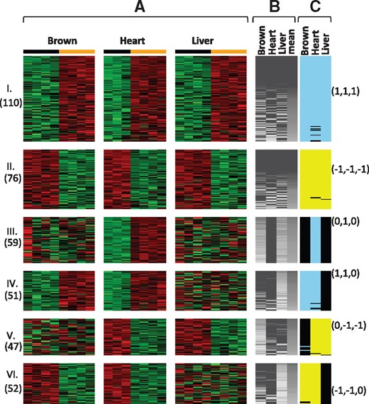
Six meta-pattern modules of biomarkers from mouse metabolism example. Each gene module (Modules I, II, …, VI) shows a set of detected biomarkers with similar meta-pattern of differential signals. (A) Heatmaps of detected genes (on the rows) and samples (on the columns) for each tissue (brown fat, heart, liver), where each tissue represents a study. In the heatmap, red color represents higher expression level, and the green color represents lower expression level. Black color bar on top represents wild-type (control) and orange color bar on top represents VLCAD−/− mice (case). Number of genes is shown on the left under each module number. (B) Variability index (genes on the rows and studies on the columns). Variability index is described in Section 2.2. Gray heatmap range from 0 (black) to 1 (white), which is the maximum of the variability index. Genes of each module are sorted based on the mean variability index. (C) Signed AW-Fisher weights ${\widehat{v}}_{\mathit{gk}}$ for gene g and study k. Light blue represents$\mathrm{ }{\widehat{v}}_{\mathit{gk}}=1$⁠, yellow corresponds to ${\widehat{v}}_{\mathit{gk}}=-1$ and black for$\mathrm{ }{\widehat{v}}_{\mathit{gk}}=0$⁠. Representative signed AW-Fisher weights for each module are shown on the right. Note brown represents brown fat tissue. (Color version of this figure is available at Bioinformatics online.)

Our methods aim to solve these issues of the AW-Fisher’s method. The performance will be evaluated in both simulations and real data applications.

2 Materials and methods

2.1 Fast computation of AW-Fisher

In this section, we provide solutions to the two computational problems mentioned in Issue 1. We propose a fast algorithm of searching the adaptive weights and an interpolation approach to obtain accurate P-values. In Supplementary Section SI, we also derive closed-form solution for the cases K = 2 to benchmark the performance of the proposed method, and K = 3 for the purpose of demonstrating difficulties of deriving closed-form solution in general K.

Recall that the AW-Fisher method $T({\displaystyle \overrightarrow{\mathbf{P}}};{\displaystyle \overrightarrow{\mathbf{w}}})=-2{\sum }_{k=1}^K{w}_k\mathrm{l}\mathrm{og}{P}_k$ belongs to HS_B, which targets on biomarkers DE in one or more studies (⁠$H_0:{\displaystyle \overrightarrow{\theta }}\in \cap \{{\mathrm{\theta }}_k=0\}$ versus$\mathrm{ }{H}_A:{\displaystyle \overrightarrow{\theta }}\in \cup \{{\mathrm{\theta }}_k\ne 0\}$⁠). The search space $\mathrm{\Omega }=\{{\displaystyle \overrightarrow{\mathbf{w}}}:{\displaystyle \overrightarrow{\mathbf{w}}}\ne 0,{\displaystyle \overrightarrow{\mathbf{w}}}=(w_1,\dots ,w_K)\in {\{0, 1\}}^K\}$ contains $2^K-1$ non-zero vectors of weights and searching the whole space Ω to find the AW-Fisher test statistic $s\left({\displaystyle \overrightarrow{\mathbf{P}}}\right)={\min }_{\overrightarrow{w}\in \mathrm{\Omega }}L\left(T\right({\displaystyle \overrightarrow{\mathbf{P}}};{\displaystyle \overrightarrow{\mathbf{w}}}\left)\right)$ and the adaptive weights $w\left({\displaystyle \overrightarrow{\mathbf{P}}}\right)=\arg {\min }_{{\displaystyle \overrightarrow{\mathbf{w}}}\in \mathrm{\Omega }}L\left(T\right({\displaystyle \overrightarrow{\mathbf{P}}};{\displaystyle \overrightarrow{\mathbf{w}}}\left)\right)$ becomes computationally expensive when K is large. The amount of computation is even more challenging when the AW-Fisher’s method is applied to genomic data, where the same procedure is repeated for thousands of genes or even millions of single nucleotide polymorphisms. To overcome this difficulty, we propose a fast algorithm to find $\widehat{\mathbf{w}}$ based on the ordered P-values ${\left\{P_{\left(i\right)}\right\}}_{i=1}^K$ with$\mathrm{ }{P}_{\left(1\right)}\le \dots \le P_{\left(K\right)}$⁠. Specifically, by decomposing Ω into $\mathrm{\Omega }=\underset{k=1}{\overset{K}{\cup }}{\mathrm{\Omega }}_k$ with$\mathrm{ }{\mathrm{\Omega }}_k=\{{\displaystyle \overrightarrow{\mathbf{w}}}:{\sum }_{j=1}^K{w}_j=k\}$⁠, it can be seen that$s\left({\displaystyle \overrightarrow{\mathbf{P}}}\right)={\min }_{{\displaystyle \overrightarrow{\mathbf{w}}}\in \Omega }\left\{L\right(T({\displaystyle \overrightarrow{\mathbf{w}}};{\displaystyle \overrightarrow{\mathbf{P}}})\left)\right\}={\min }_{1\le k\le K}{\min }_{{\displaystyle \overrightarrow{\mathbf{w}}}\in {\mathrm{\Omega }}_k}\left\{L\right(T({\displaystyle \overrightarrow{\mathbf{w}}};{\displaystyle \overrightarrow{\mathbf{P}}})\left)\right\}$⁠. Given $1\le k_0\le K$⁠, denote by ${{\displaystyle \overrightarrow{\mathbf{w}}}}^{k_0}=({w_1}^{k_0},\dots ,{w_K}^{k_0})$ the vector of weights such that $-2{\sum }_{j=1}^K{w_j}^{k_0}\mathrm{l}\mathrm{og}\left(P_j\right)=-2{\sum }_{j=1}^{k_0}\log \left(P_{\left(j\right)}\right)$ (i.e. the Fisher’s statistic using the first k₀ smallest P-values). Then it is straightforward to see that the test statistic involving the first k₀ ordered P-values will generate the most significant $L\left(T\right({\displaystyle \overrightarrow{\mathbf{P}}};{\displaystyle \overrightarrow{\mathbf{w}}}\left)\right)$ in $\mathrm{ }{\mathrm{\Omega }}_{k_0}$⁠. This implies in $\mathrm{ }{\mathrm{\Omega }}_{k_0}$⁠, only ${{\displaystyle \overrightarrow{\mathbf{w}}}}^{k_0}$ has to be considered for further comparison. Therefore, instead of searching the whole space Ω, it is enough to search only K vectors of weights $\{{{\displaystyle \overrightarrow{\mathbf{w}}}}^1,\dots ,{{\displaystyle \overrightarrow{\mathbf{w}}}}^K\}$ to find the adaptive weights $\mathrm{ }\widehat{\mathbf{w}}$⁠. The proposed fast algorithm contains two steps: first sorting K P-values [usually with complexity of$\mathcal{ }\mathcal{O}\left(K\log \right(K\left)\right)$] and then searching K vectors of weights (with complexity of$\mathcal{ }\mathcal{O}\left(K\right)$⁠). Therefore, the fast searching algorithm proposed in this section reduces the computational complexity from $\mathcal{O}\left(2^K\right)$ to$\mathcal{ }\mathcal{O}\left(K\log \right(K\left)\right)$⁠, which can significantly reduce computing time when K is large.

Denote by ${{\displaystyle \overrightarrow{\mathbf{p}}}}_{\mathrm{obs}}$ the observed P-values from individual studies and $s_{\mathrm{obs}}=s\left({{\displaystyle \overrightarrow{\mathbf{p}}}}_{\mathrm{obs}}\right)$ the observed AW-Fisher statistic. Theoretically, the P-value of the AW-Fisher’s method ${\mathbb{P}}_{H_0}(S\le s_{\mathrm{obs}})$ can be calculated analytically for any $K\ge 2$⁠. However, the formulae involve the evaluation of a K-fold integral and the integration domain becomes very complicated for $K\ge 3$⁠, which makes the derivation of the closed-form solution tedious and fallible. For illustration, closed-form derivation of K = 2 and K = 3 are shown in Supplementary Section SI. In Li and Tseng (2011), a permutation test by randomly permuting class labels in each study was proposed. Although this non-parametric approach has its merit of maintaining gene dependency structure, it is computationally demanding and difficult for generating precise small P-value, such as when P-value$<{10}^{-4}$⁠, which is a critical requirement for multiple testing correction on thousands of genes. In this paper, we propose to use importance sampling to obtain an accurate numerical approximation of $\mathrm{ }{\mathbb{P}}_{H_0}(S\le s_{\mathrm{obs}})$⁠. Importance sampling is a method to accurately estimate the expectation of a function with very small value using Monte Carlo sampling. The idea behind importance sampling is to draw samples from a suitable new distribution function rather than the original one of interest and assign a weight to each sample based on the ratio of two density functions.

To evaluate AW-Fisher P-value ${\mathbb{P}}_{H_0}(S\le s_{\mathrm{obs}})$ using importance sampling, we propose a beta-distribution density function $f^{*}(·)$ to draw ${\displaystyle \overrightarrow{\mathbf{P}}}$ instead of natural uniform distribution f(⋅) so that we can ‘over-sample’ those small P-values that result in a large S. It holds that

$${\mathbb{P}}_{H_0}(S\le s_{\mathrm{obs}})={\mathbb{E}}_{H_0}\left[\mathbb{I}\right\{S\le s_{\mathrm{obs}}\left\}\right]=\int \mathbb{I}\{S\le s_{\mathrm{obs}}\}f\left({\displaystyle \overrightarrow{\mathbf{P}}}\right)d{\displaystyle \overrightarrow{\mathbf{P}}}=\int \mathbb{I}\{S\le s_{\mathrm{obs}}\}\frac{f\left({\displaystyle \overrightarrow{\mathbf{P}}}\right)}{f^{*}\left({\displaystyle \overrightarrow{\mathbf{P}}}\right)}{f}^{*}\left({\displaystyle \overrightarrow{\mathbf{P}}}\right)d{\displaystyle \overrightarrow{\mathbf{P}}}={\mathbb{E}}^{*}\left[\mathbb{I}\right\{S\le s_{\mathrm{obs}}\}\times W({\displaystyle \overrightarrow{\mathbf{P}}}\left)\right],$$

(2)

where f(⋅) is the density of ${\displaystyle \overrightarrow{\mathbf{P}}}$ under the null and $f^{*}(·)$ is the proposed density function of ${\displaystyle \overrightarrow{\mathbf{P}}}$ for importance sampling. Importance sampling weight $W(·)=f(·)/f^{*}(·)$⁠, $\mathbb{E}(·)$ and ${\mathbb{E}}^{*}(·)$ are the expectation with respect to f(⋅) and $f^{*}(·)$ respectively. Therefore, we can obtain expectation from the original measure using a more efficient new one by applying weights for different samples in Monte Carlo method. Under the null hypothesis and independence assumption between different studies, $P_k\sim \text{UNIF}(0, 1)$ for all$1\le k\le K$⁠, so the joint distribution of $f\left({\displaystyle \overrightarrow{\mathbf{P}}}\right)=1$⁠. If we instead use $\text{Beta}(\mathrm{\eta }, 1)$ distribution as the proposed distribution of each study for importance sampling, then$\mathrm{ }{f}^{*}\left({\displaystyle \overrightarrow{\mathbf{P}}}\right)={\mathrm{\eta }}^K{\left({\prod }_{k=1}^K{P}_k\right)}^{\mathrm{\eta }-1}$⁠. To implement importance sampling, suppose we simulate $\mathrm{ }{{\displaystyle \overrightarrow{p}}}_i=(p_{i1},\dots ,p_{\mathit{iK}})$⁠, where $p_{\mathit{ik}}{\displaystyle \stackrel{\mathrm{i}.\mathrm{i}.\mathrm{d}.}{\sim }}\text{Beta}(\mathrm{\eta }, 1)$ for $1\le i\le n$ and$1\le k\le K$⁠. Denote by$\mathrm{ }{s}_i=s\left({{\displaystyle \overrightarrow{p}}}_i\right)$⁠. From Equation (2), we calculate estimate of ${\mathbb{P}}_{H_0}(S\le s_{\mathrm{obs}})$ by

$${\widehat{\mathbb{P}}}_{H_0}(S\le s_{\mathrm{obs}};\mathrm{\eta }, {{\displaystyle \overrightarrow{p}}}_1,\dots , {{\displaystyle \overrightarrow{p}}}_n)=\frac{1}{n}·\sum _{i=1}^n\left(\mathbb{I}\right\{s_i\le s_{\mathrm{obs}}\}·\frac{1}{{\eta }^K{\left({\prod }_{k=1}^K{p}_{\mathit{ik}}\right)}^{\mathrm{\eta }-1}}).$$

(3)

Our P-value evaluation procedure (also see the flowchart in Supplementary Fig. S1) has the following steps:

1. For a targeted number of studies K and target P-value c, calculate its AW-Fisher test statistic.

   • (Identify suitable η for given c_t and K): Note that different η can provide better importance sampling for different range of targeted c_t given K. When η = 1, the importance sampling method reduces to the naive Monte Carlo method. To identify an appropriate η given c_t and K, we simulate ${{\displaystyle \overrightarrow{q}}}_i=(q_{i1},\dots ,q_{\mathit{iK}})$⁠, where $1\le i\le 1000$ and $q_{\mathit{ik}}{\displaystyle \stackrel{\mathrm{i}.\mathrm{i}.\mathrm{d}.}{\sim }}\text{Unif}(0, 1)$⁠. Denote by ${q_i}^{1/\mathrm{\eta }}=({{{\displaystyle \overrightarrow{q}}}_{i1}}^{1/\mathrm{\eta }},\dots ,{q_{\mathit{iK}}}^{1/\mathrm{\eta }})$ with element-wise power to $1/\mathrm{\eta }$ and ${r_i}^{\left(\mathrm{\eta }\right)}=s\left({{{\displaystyle \overrightarrow{q}}}_i}^{1/\mathrm{\eta }}\right)$⁠. Define $r_0={\text{median}}_{1\le i\le 1000}\left({r_i}^{\left(\mathrm{\eta }\right)}\right)$⁠. Note that since$\mathrm{ }{q}_{\mathit{ik}}{\displaystyle \stackrel{\mathrm{i}.\mathrm{i}.\mathrm{d}.}{\sim }}\text{Unif}(0, 1)$⁠, $q_{\mathit{iK}}^{1/\mathrm{\eta }}\sim \text{Beta}(\mathrm{\eta },1)$⁠. From Equation (3), we have

     $$\begin{array}{c}\varphi (\eta )={\widehat{\mathbb{P}}}_{H_0}(S\le r_0;\eta , {{{\displaystyle \overrightarrow{q}}}_i}^{1/\mathrm{\eta }},\dots ,{{{\displaystyle \overrightarrow{q}}}_{1000}}^{1/\mathrm{\eta }})\\ =\frac{1}{1000}·\sum _{i=1}^{1000}\left(\mathbb{I}\left\{r_i^{\left(\eta \right)}\le r_0\right\}·\frac{1}{{\eta }^K{\left({\prod }_{k=1}^K{{\stackrel{}{q}}_{\mathit{iK}}}^{1/\mathrm{\eta }}\right)}^{\mathrm{\eta }-1}}\right).\end{array}$$

     (4)

     We choose $\mathrm{\eta }(K,c_t)$ as the root of $\mathrm{\varphi }\left(\mathrm{\eta }\right)=c_t$⁠, which can be numerically obtained using ‘uniroot()’ function in R. This choice of η guarantees half of the simulated samples will effectively contribute to the importance sampling calculation for each targeted c_t. Alternatively, one can choose η by minimizing the variance (i.e. find η such that $\mathrm{Va}{\mathrm{r}}_{H_0}\left[\mathbb{I}\right\{S\le s_{\mathrm{obs}}\left\}\right]$ is minimized). However, for$\mathrm{ }{c}_t\ge 0.01$⁠, we set η = 1 since the gain of importance sampling diminishes.
   • (Derive corresponding AW-Fisher statistic for targeted P-value c_t): Next, we derive the corresponding AW-Fisher statistic $S_{K,t}$ for a targeted P-value c_t given K. Given K and c_t, we use $\mathrm{\eta }(K,c_t)$ (abbreviated as η hereafter) from the previous step to draw $\mathrm{ }{{\displaystyle \overrightarrow{o}}}_i=(o_{i1},\dots ,o_{\mathit{iK}})$⁠, where $1\le i\le {10}^7$ and$\mathrm{ }{{\displaystyle \overrightarrow{o}}}_i{\displaystyle \stackrel{\mathrm{i}.\mathrm{i}.\mathrm{d}.}{\sim }}\text{Beta}(\mathrm{\eta },1)$⁠. Denote by $t_i=s\left({{\displaystyle \overrightarrow{o}}}_i\right)$ the corresponding AW-Fisher statistic of ${{\displaystyle \overrightarrow{o}}}_i$ and $t_{\left(1\right)}\le t_{\left(2\right)}\le \dots \le t_{\left({10}^7\right)}$ are ordered from $\mathrm{ }{t}_1,\dots ,t_{{10}^7}$⁠. Define

     $$\begin{array}{c}{m}_i={\widehat{\mathbb{P}}}_{H_0}(S\le t_{\left(i\right)};\eta ,{{\displaystyle \overrightarrow{o}}}_1,\dots ,{{\displaystyle \overrightarrow{o}}}_{{10}^7})\\ =\frac{1}{{10}^7}·\sum _{j=1}^{{10}^7}\left(\mathbb{I}\left\{t_j\le t_{\left(i\right)}\right\}·\frac{1}{{\mathrm{\eta }}^K{\left({\prod }_{k=1}^K{o}_{\mathit{jk}}\right)}^{\mathrm{\eta }-1}}\right).\end{array}$$

     (5)

     Note that m_i is monotonically increasing with respect to i and $m_1\approx 0$⁠. There exists $i^{*}$ such that$\mathrm{ }{m}_{i^{*}}\le c_t<m_{i^{*}+1}$⁠. The corresponding AW-Fisher statistic $S_{K,t}$ given K and c_t is chosen as $S_{K,t}=t\left(i^{*}\right)$⁠.

2. Specify a grid of targeted $K=2, 3, \dots , 100$ and targeted AW-Fisher P-values as $\{c_t,t=1, 2, \dots , 198\}=\{1, 0.99, 0.98,0.97, \dots , 0.03, 0.02, 0.01,{10}^{-3},{10}^{-4},{10}^{-5},\dots ,{10}^{-100}\}$⁠.

3. (Interpolation to calculate P-value of a given S_obs): From Step 1b, the library of c_t and $S_{K,t} (t=1,\dots ,198\mathrm{and}\mathrm{ }K=2,\dots ,100)$ is established for interpolation. For any given AW-Fisher statistic S_obs and K, we apply function splinefun in R with monoH.FC option using $\left(\log \right(S_{K,t}), \log (c_t\left)\right)$⁠, where $t=1, 2,\dots , 198$⁠, to fit a smooth curve and identify the corresponding P-value of S_obs. Note that we apply spline on log-scale P-value to avoid numerical overflow.

 

Remark. In Step 1a, given K, we simulate $q_{\mathit{ik}}{\displaystyle \stackrel{\mathrm{i}.\mathrm{i}.\mathrm{d}.}{\sim }}\text{Unif}(0, 1)$  and take the power of $1/\mathrm{\eta }$, instead of simulating from$\text{Beta}(\mathrm{\eta },1)$. This design guarantees $\mathrm{\varphi }\left(\mathrm{\eta }\right)$  is a monotone function with respect to η by eliminating the uncertainty from sampling q_ik for each η.

For any future input P-values, we only need to calculate the AW-Fisher statistics and interpolate the statistics to obtain AW-Fisher P-value by the spline curve fitting. The design of our base library$\left\{\right(\log \left(S_{K,t}\right),\log \left(c_t\right))$⁠; $(t=1,\dots ,198,$ and $K=2,\dots ,100\left)\right\}$ facilitates accurate estimation for the AW-Fisher P-value in the range of $({10}^{-100},1)$ and K up to 100. Although the computation is demanding to generate the base library, it only runs once before we generate our AW-Fisher R package and will not affect computing for users. In fact, as shown in Section 3.1.1, the new approach is even faster than closed-form solution once the base library in the R package is established.

2.2 Variability index of adaptive weights

As discussed in Issue 2 in the Section 1, the AW weight estimate ${\widehat{w}}_g=({\widehat{w}}_{g1},\dots ,{\widehat{w}}_{\mathit{gK}})$ is discontinuous as a function of the input P-values and thus may not be stable. Denote by $U_{\mathit{gk}}=4· \text{Var}\left({\widehat{w}}_{\mathit{gk}}\right)$ the variability index of the AW weight estimate for gene g in study k, where the normalization factor 4 scales $U_{\mathit{gk}}$ to range within$[0, 1]$⁠. The variability index gauges the stability of $\mathrm{ }{\widehat{w}}_{\mathit{gk}}$⁠, where a smaller variability index indicates a stable AW weight estimate. However, $U_{\mathit{gk}}$ is not easy to evaluate since ${\widehat{w}}_{\mathit{gk}}$ is binary. Here, we propose a bootstrap procedure to calculate an estimate of $\mathrm{ }{U}_{\mathit{gk}}$⁠. The procedure is as follows:

1. Obtain a bootstrap sample and repeat the following procedure B (⁠$b=1,\dots ,B$⁠) times. Denote by $D_k\in {\mathbb{R}}^{G\times N_k}$ the data matrix of study k, where G is the total number of genes and N_k is the total number of samples for study k. c_ki is the case–control label, where $i\in \{1,\dots ,N_k\}$ is the sample index and c_ki = 0 or 1, representing sample i belongs to control or case group. Perform bootstrapping by resampling columns with replacements within case and control, respectively. To be specific, we create an empty data matrix ${D_k}^{\left(b\right)}\in {\mathbb{R}}^{G\times N_k}$⁠. Then sample the ith column of ${D_k}^{\left(b\right)}$ using jth column of D_k, where $j\in \{j\text{'}:c_{\mathit{kj}\text{'}}=c_{\mathit{ki}}\}$⁠. This bootstrap procedure is stepped through for $i=1,\dots ,N_k$ with replacement (allowing ${D_k}^{\left(b\right)}$ as identical columns). Use bootstrapped data matrix ${D_k}^{\left(b\right)}$ to generate an AW weight estimate ${{\widehat{w}}_{\mathit{gk}}}^{\left(b\right)}$ and an effect size estimate ${{\widehat{\mathrm{\theta }}}_{\mathit{gk}}}^{\left(b\right)}$⁠. Calculate the variability index estimate ${\widehat{U}}_{\mathit{gk}}$ of ${\widehat{w}}_{\mathit{gk}}$ for gene g in study k, where $\mathrm{ }{\widehat{U}}_{\mathit{gk}}=\frac{4}{B}{\sum }_{b=1}^B{({{\widehat{w}}_{\mathit{gk}}}^{\left(b\right)}-\frac{1}{B}{\sum }_{b\text{'}=1}^B{{\widehat{w}}_{\mathit{gk}}}^{\left(b\text{'}\right)})}^2$⁠.

Here ${\widehat{U}}_{\mathit{gk}}$ ranges from 0 to 1 with ${\widehat{U}}_{\mathit{gk}}=0$ represents ${{\widehat{w}}_{\mathit{gk}}}^{\left(b\right)}={\widehat{w}}_{\mathit{gk}}$ for all b, which indicates stable estimate of the AW weight since its bootstrap variance is 0. ${\widehat{U}}_{\mathit{gk}}=1$ represents ${{\widehat{w}}_{\mathit{gk}}}^{\left(b\right)}=0$ for half of $b\text{'}s$ and ${{\widehat{w}}_{\mathit{gk}}}^{\left(b\right)}=1$ for the other half of $b\text{'}s$⁠. A large variability index indicates an unstable estimate of the AW weight.

2.3 Resampling-based ensemble clustering for biomarker categorization

In order to categorize detected genes into biomarker groups with similar differential meta-pattern (Issue 3), we extended the bootstrapping procedure in Section 2.2 to obtain a co-membership matrix for all pairs of genes where each element of the co-membership matrix represents a similarity of signed AW weight $\widehat{\mathbf{v}}$ of two genes. Specifically, denote by ${{\widehat{v}}_{\mathit{gk}}}^{\left(b\right)}={{\widehat{w}}_{\mathit{gk}}}^{\left(b\right)}·\text{sign}\left({{\widehat{\mathrm{\theta }}}_{\mathit{gk}}}^{\left(b\right)}\right)$ from Section 2.2. Define co-membership matrix from each bootstrap sample b as $W^{\left(b\right)}\in {\mathbb{R}}^{G\times G}$ with elements ${W_{\mathit{gg}\text{'}}}^{\left(b\right)}=1$ if ${{\widehat{v}}_{\mathit{gk}}}^{\left(b\right)}={{\widehat{v}}_{g\text{'}k}}^{\left(b\right)}$ for all k, and ${W_{\mathit{gg}\text{'}}}^{\left(b\right)}=0$ otherwise. The final co-membership matrix is defined as $V={\sum }_{b=1}^B{W}^{\left(b\right)}/B$⁠. We further applied the tight clustering algorithm (Tseng and Wong, 2005) (tight.clust function within R package tightClust) using the co-membership matrix V to obtain tight modules. Tight clustering is able to produce tight and stable gene modules without forcing all genes into clusters. Note that for the clustering algorithm, the dissimilarity measure between two genes i and j can be calculated as $\mathrm{ }{d}_{\mathit{ij}}=D(V_i,V_j)$⁠, where $V_i\in {\left[\mathrm{0,1}\right]}^G$ is the ith column of the co-membership matrix V and D can be any distance measurement mapping. Throughout this paper, we calculate the dissimilarity measure using the Euclidean distance $\mathrm{ }{d}_{\mathit{ij}}=\left|\right|V_i-V_j|{|}_2$⁠. The resulting gene modules show unique DE patterns across multiple studies (namely meta-pattern). We perform the biomarker categorization (clustering) procedure only on declared DE genes at certain FDR cutoff. Genes of each resulting module are then sorted by the variability index and visualized by heatmaps. Below we perform simulations to demonstrate the performance of the resampling-based ensemble clustering for biomarker categorization.

Note that based on the co-membership matrix, one can use any clustering algorithm to obtain the DE patterns. We used the tight clustering algorithm throughout this manuscript due to its capability to remove noise genes (genes that are not assigned to any cluster).

3 Results

3.1 Simulation results

3.1.1 Simulation and numerical evaluation for fast AW-Fisher computing

In Section 2.1 we introduced the fast computation for the AW-Fisher P-value via importance sampling and interpolation by spline smoothing. In this section, this interpolation approach will be compared to the original permutation-based approach in Li and Tseng (2011) and Wang et al. (2012). The comparisons include evaluation of accuracy and computing speed. In terms of computing speed, our approach applies a new linear sorting algorithm for searching weights and an interpolation for P-value calculation. The improvement of linear sorting algorithm is quite obvious: the search space reduces from an exponential order $\mathcal{O}\left(2^K\right)$ to almost linear order$\mathcal{ }\mathcal{O}\left(K\log \right(K\left)\right)$⁠. Below we utilize the closed-form solution for K = 2 (details in Supplementary Section SI.1) as the underlying truth to compare the new approach with the existing permutation approach. The linear sorting does not improve computing speed when K = 2 and the improvement will mainly come from the interpolation. The simulation setting is described in Supplementary Section SII.

Using the closed-form solution as the underlying truth, we evaluated the performance of the AW-Fisher P-value with K = 2 studies from the interpolation approach using the permutation approach as the primary baseline. Since the importance sampling method reduces to Monte Carlo method when setting η = 1 in Equation (3), we also treat the Monte Carlo method as a secondary baseline. To formally evaluate the accuracy from the permutation approach, Monte Carlo approach, or the interpolation approach, we utilized root mean square error (rMSE): $\text{rMSE}=\sqrt{{\sum }_{g=1}^{G_1}{({\mathrm{\alpha }}_g-{\mathrm{\beta }}_g)}^2/G_1},$ where α_g is the $-{\log }_{10}$ (AW-Fisher P-value) for gene g; β_g is the $-{\log }_{10}$ (AW-Fisher P-value) for gene g from closed-form solution; G₁ is the total number of genes being evaluated; and the rMSE indicates the accuracy of P-value estimates with smaller rMSE for better estimation. The result for (i) $N_1=20,\hspace{0.33em}{N}_2=20$ is shown in Table 1, the results for (ii) $N_1=50,\hspace{0.33em}{N}_2=50$ and (iii) $N_1=20,\hspace{0.33em}{N}_2=50$ are shown in Supplementary Tables S1 and S2. Our proposed interpolation approach is superior to permutation-based approach and the Monte Carlo approach in terms of accuracy. In terms of computing time, we want to de-emphasize the permutation-based approach because in some cases the per study P-values will be calculated by permutation tests, where the permutations occur anyway so that calculating the meta-analysis P-value through permutation will not incur much additional cost. However, the permutation test is not always available, for example, when sample sizes per study may be too small to perform permutation, or in a meta-analysis context one may only have access to computed P-values, but maybe not the raw data. Under these scenarios, Monte Carlo approach is more appropriate to calculate the P-value. Regardless using the permutation-based approach or the Monte Carlo approach as baseline, we observe that the interpolation approach is much faster. Note that the interpolation approach is even faster than closed-form solution because the interpolation is only based on spline curve fitting using data in the library and does not implement importance sampling method while the closed-form method requires evaluation of power and logarithmic functions.

Table 1.

AW-Fisher P-value accuracy in terms of rMSE comparing interpolation approach, permutation-based approach and Monte Carlo approach with closed-form solution as benchmark

P-value range	Interpolation	Permutation		Monte Carlo
		$B={10}^3$	$B={10}^4$	$B={10}^3$	$B={10}^4$
(0.01, 1]	0.0002	0.0031	0.0014	0.0015	0.0002
(0.001, 0.01]	0.0003	0.071	0.035	0.042	0.0047
(0.0001, 0.001]	0.0007	0.31	0.15	0.25	0.037
(1e-10, 0.0001]	0.0006	3.3	2.5	3.3	2.5
(1e-50, 1e-10]	0.0023	16.6	15.7	16.6	15.7
(1e-100, 1e-50]	0.0069	59.1	58.1	59.1	58.1
Time	0.011 s	18.5 min	2.1 h	9.5 min	1.6 h

Note: Two studies (sample size$\mathrm{ }{N}_1=20,\hspace{0.33em}{N}_2=20$⁠) are included as input. B is the number of permutations/samplings, and the closed-form solution and the interpolation approach do not require any permutation. The range of the resulting AW-Fisher P-values is displayed in the first column. The computing time for each method is displayed in the last row. The computing time for the closed-form solution is 0.06 s.

To further evaluate whether our proposed method can well control the Type I error rate, we have included QQ plots as well as estimated Type I errors at various levels under the null. From the QQ plots (Supplementary Figs S2, S3 and S4), we can see the genomic inflation factors ranging from 0.999 to 1.001, indicating that the Type I error rate is well controlled. From the Type I error rate estimation table (Supplementary Table S3), we observe that the Type I error rate is correctly estimated around their nominal level, further corroborating the accurate Type I error rate control of the proposed interpolation method.

3.1.2 Simulation results for the variability index

The main simulation setting mimics a transcriptomic study by considering generative process of DE genes and correlation structures between genes. The procedure generally follows Song and Tseng (2014). Note that this simulation also applies to Section 3.1.1. Details of the simulation procedure are in Supplementary Section SII.

To evaluate the performance of the variability index, we considered different combinations of biological variance (⁠$\mathrm{\sigma }=1, 1.5, 2$⁠) and sample sizes (N = 20, 50, 80). The result in Supplementary Figure S5 shows that when the dataset has smaller sample size or larger biological variation, the variability index becomes larger. Since the variability index gauges the stability of the AW weight estimate, it can be seen that noisy datasets tend to generate large variability index. In addition, we drew bar plot of the variability index with respect to true positive (TP), false positive (FP) and false negative (FN). As shown in Supplementary Figure S6, FN has larger variability index, followed by FP, and lastly TP, under different scenarios of sample sizes and noise level, which is expected since the weight of TPs are likely to be stable, and the weight of FP and FN are on the decision boundary, and thus unstable. The scatter plots of P-value and the variability index are shown in Supplementary Figure S7. We observed that with respect to the increase of $-{\log }_{10}(P-\mathrm{value})$⁠, the variability index goes up, and finally goes down to zero.

3.1.3 Simulation result for biomarker categorization

To evaluate the performance of biomarker categorization, we adopted a simulation procedure similar to Section 3.1.2 and Huo et al. (2019). We simulated K = 4 studies in total and 50 control subjects and 50 case subjects in each study. Among the G = 10 000 genes, we set 4% as homogeneously concordant DE genes, DE with the same direction in all studies (all positive or all negative). We denote ‘homo+’ as the homogeneously concordant DE genes with all positive effect sizes and ‘homo−’ as the homogeneously concordant DE genes with all negative effect sizes. We also set another 4% as study-specific DE genes—differential expressed only in one study. Among them, 1/4 are DE genes only in the first study with positive effect sizes (denoted as ‘ssp1+’), 1/4 are DE genes only in the first study with negative effect sizes (denoted as ‘ssp1−’), 1/4 are DE genes only in the second study with positive effect sizes (denoted as ‘ssp2+’), and the rest 1/4 are DE genes only in the second study with negative effect sizes (denoted as ‘ssp2−’). The rest of the genes are non-DE (denoted as ‘non-DE’). The biological variation parameter σ is set to 1 in this simulation.

By applying the AW-Fisher method, we obtained 794 genes based on FDR at 5% under HS_B$\mathrm{ }{\mathit{HS}}_B$⁠. Co-membership of these genes were calculated with B = 1000 and used as input for our gene module detection using the tight clustering algorithm. We identified 6 gene modules in these 794 genes. The detected gene modules are tabulated against the true gene modules simulated in Table 2 (Module 0 contains scattered genes not assigned to any of the six modules). The FDR is well controlled at $34/794=4.3\%$ while the nominal FDR is 5%. The detected gene modules clearly correspond to the true modules, and most of the non-DE genes were left out as the noises. The meta-pattern, variability index and AW weight estimates of these six modules are shown in Supplementary Figure S8. This simulation study showed that the proposed algorithm can recover the underlying gene meta-pattern.

Table 2.

Contingency table of 794 detected DE genes with simulation underlying truth (on the columns) and the tight clustering result with 6 target modules (on the rows)

Module	homo−	homo+	ssp1−	ssp1+	ssp2−	ssp2+	Non-DE
1	0	177	0	0	0	0	0
2	184	0	0	0	0	0	0
3	0	0	0	74	0	0	1
4	0	0	60	0	0	0	1
5	0	0	0	0	0	102	2
6	0	0	0	0	85	0	3
0	13	24	19	11	6	5	27

Note: 0 represents the scattered gene group. 1 ∼ 6 represent 6 detected modules. Bolded numbers are genes with correct assignment.

Based on the co-membership matrix, we can perform any clustering algorithm to obtain the gene meta-pattern. Hence, we also applied K-means and hierarchical clustering for comparison. The confusion tables of the resulting gene modules and the underlying true gene modules are shown in Supplementary Tables S4 and S5. In order to benchmark the results, we adopted the adjusted Rand index (Hubert and Arabie, 1985), which is a measure for the similarity between two clustering assignment results (ranges from 1 to −1), with larger number indicating better consistency. Compared to the underlying truth, the adjusted Rand index for tight clustering, K-means and hierarchical clustering are 0.83, 0.82 and 0.80, respectively.

3.2 Transcriptomic meta-analysis applications

3.2.1 Mouse metabolism example

Very long-chain acyl-CoA dehydrogenase (VLCAD) deficiency was found to be associated with energy metabolism disorder in children. Two genotypes of the mouse model—wild-type (VLCAD +/+) and VLCAD-deficient (VLCAD −/−)—were studied for four types of tissues (brown fat, liver, heart and skeleton) with 3–4 mice in each genotype group. In order to better demonstrate the biological interpretability of the proposed method, we focused on the first three tissues (brown fat, liver and heart) as our primary analysis. We also analyzed all four tissues in order to demonstrate when the number of studies K is large, the biomarker categorization based on the unique AW weight estimate becomes infeasible but our proposed method is much more tractable. Total number of probesets from these three transcriptomic microarray studies is 14 495. Supplementary Table S6a shows details of the study design. Two-sided P-values and effect sizes were calculated using limma comparing wild-type (VLCAD +/+) versus mutant (VLCAD −/−) mice in each tissue. AW-Fisher meta-analysis P-values were obtained and q-values were calculated by applying Benjamini–Hochberg procedure. By controlling FDR at 5%, we obtained 967 DE genes. We calculated the variability index and generated gene co-membership matrix using resampling techniques. We further applied the tight clustering algorithm on the co-membership to identify gene modules with unique meta-pattern. In this example, we successfully detected six gene modules with different meta-patterns in Figure 1. For example, the first and second biomarker modules (Gene clusters I and II) are concordant genes that are up-regulated (or down-regulated) in all tissues. The other biomarker modules have study-specific differential patterns. For example, DE genes in Gene module III are up-regulated in heart but not in brown fat or liver. To examine the biological functions of these modules, we performed pathway enrichment analysis for genes in each module using Fisher’s exact test. The pathway database was downloaded from Molecular Signatures Database (MSigDB) v5.0 (http://bioinf.wehi.edu.au/software/MSigDB/), where a mouse-version pathway database was created by combining pathways from KEGG, BIOCARTA, REACTOME and GO databases and mapping all the human genes to their orthologs in mouse using the Jackson Laboratory Human and Mouse Orthology Report (http://www.informatics.jax.org/orthology.shtml). Among the six gene modules with distinct meta-patterns, Module I is enriched in enzyme activities (e.g. GO COFACTOR BINDING;$p=3.85\times {10}^{-4}$⁠); Module II is enriched in pathways for amino acid catabolism (e.g. REACTOME BRANCHED CHAIN AMINO ACID CATABOLISM;$p=9.31\times {10}^{-5}$⁠); Module III is enriched in defense related pathways (e.g. DEFENSE RESPONSE;$p=2.11\times {10}^{-6}$⁠); Module IV is enriched in pathways of metabolism of amino acids (e.g. REACTOME METABOLISM OF AMINO ACIDS;$p=2.36\times {10}^{-3}$⁠); Module V is enriched in stimulus related pathways (e.g. EXTERNAL STIMULUS;$p=1.33\times {10}^{-3}$⁠); For Module VI, we did not detect any significantly enriched pathways. Interestingly, all of these pathways are known to be related to different aspects of metabolism, which indicates that our method is able to detect homogeneous and heterogeneous gene modules that are biologically meaningful. Such biomarker categorizations may help enhance meta-analysis interpretations and motivate further biological hypotheses. For example, it is intriguing why the defense related genes in Module III are up-regulated only in heart but not in liver and brown fat, and why the stimulus related genes in Module V are down-regulated in heart and liver but not in brown fat. Among the six detected meta-pattern modules, 5 (83%) of them are biologically interpretable (defined as genes in the module are statistically enriched using Fisher’s exact test with P-value < 0.005 in at least one pathway). In contrast, the biomarker categorization based on the unique AW weight estimate is hard to characterize as there are $3^3-1=26$ modules. In addition, among these modules only 13 (50%) are significantly enriched in at least one pathway with P-value < 0.005.

In order to benchmark the improvement of computational speed and feasibility, we also applied the original permutation approach (Li and Tseng, 2011) with number of permutation B = 1000. The entire analysis from raw data only took our proposed method 0.34 s while the permutation approach required 6.57 min.

The variability index helps characterize the instability of the AW weight estimate. Supplementary Table S7 listed 11 genes with similar P-values, but their AW weight estimates in the second study (heart) can be different since their AW variabilities are large. For example, P-values for probeset $1419484\_a\_\mathit{at}$ were $(0.00039,0.096, 0.0021)$ and its AW weight estimates were $\mathrm{ }\widehat{w}=(1, 1, 1)$⁠, while P-values for probeset $1425567\_a\_\mathit{at}$ were $(0.00036,0.10, 0.0021)$ and its AW weight estimates were $\mathrm{ }\widehat{w}=(1, 0, 1)$⁠. The variability index of $\widehat{w}=(1, 1, 1)$ in $1419484\_a\_\mathit{at}$ is (0, 0.93, 0) and variability index of $\widehat{w}=(1, 0, 1)$ in $1425567\_a\_\mathit{at}$ is (0, 0.94, 0), showing unstable weight estimate of the second study for both gene probes.

In addition, we drew scatter plots of P-value and the variability index in Supplementary Figure S9. Similar to what has been observed in the simulation, with respect to the increase of $-{\log }_{10}(P-\mathrm{value})$⁠, the variability index goes up, and finally goes down to zero. This is also expected because the weight on the boundary (with moderate P-values) tends to be FP and FN, which has larger variability. The extreme significant P-values provide strong evidence to be TP, and thus have 0 variability.

Following the same procedure, we further applied the proposed method on all four tissues. 1073 DE genes were detected at FDR 5%. The resulting meta-pattern visualization is shown in Supplementary Figure S10. Among the top 10 detected meta-pattern modules, 8 (80%) of them were biologically interpretable. In contrast, the biomarker categorization based on the original AW weight estimate was intractable, since it produced $3^4-1=80$ modules. In addition, among these modules, only 26 (33%) were significantly enriched in at least one pathway with P-value < 0.005.

3.2.2 HIV transgenic rat RNA-seq data

Li et al. (2013) conducted studies to determine gene expression differences between F344 and HIV transgenic rats using RNA-seq (GSE47474 in Gene expression Omnibus database. The HIV transgenic rat model is designed to study learning, memory and vulnerability to drug addiction and other psychiatric disorders to HIV positive patients. Twelve F334 untreated rats and 12 HIV transgenic rats in prefrontal cortex (PFC), hippocampus (HIP) and striatum (STR) regions are sequenced for RNA-seq (see Supplementary Table S6b). Tophat (Trapnell et al., 2009) was applied for alignment (adopted by Li et al., 2013) and the alignment results were converted to RNA-seq count data with 16 821 genes by BEDTools (Quinlan and Hall, 2010). Genes with <100 total counts within any brain region were filtered out and 11 824 genes remained. Potential outliers were removed by checking the sample correlation heatmaps (see Supplementary Fig. S11). R package edgeR (Robinson et al., 2010) was adopted to perform differential expression gene detection and two-sided P-values were obtained. AW-Fisher meta-analysis P-values were evaluated and q-values were obtained by applying the Benjamini–Hochberg procedure. By controlling FDR at 30%, we obtained 145 DE genes. We loosen the FDR criteria to 30% since it is well known that the transcriptomic signals in brain are generally weak. We calculated the variability index and performed biomarker categorization by using resampling techniques and the tight clustering algorithm. The result is shown in Supplementary Fig. S12. To examine the biological functions of these modules, we also performed pathway enrichment analysis using the same procedure as in Section 3.2.1. As the results show, Module I is up-regulated in all the three brain regions, and is enriched in pathways related to response to virus (e.g. GO RESPONSE TO VIRUS;$p=1.59\times {10}^{-3}$⁠); Module II is down-regulated in all the three brain regions, and is enriched in pathways related to rhythmic process (e.g. GO RHYTHMIC PROCESS;$p=6.23\times {10}^{-4}$⁠); Module III is especially interesting since it is down-regulated in HIP, but up-regulated in PFC and STR. It is enriched in transporter related pathways (e.g. REACTOME INORGANIC CATION ANION SLC TRANSPORTERS; $p=3.67\times {10}^{-3}$⁠). Since the brain is responsive for the virus invasion, we anticipate that genes responding to virus to be up-regulated, as observed in Module I. The down-regulation of rhythmic process genes in Module II indicates that HIV virus may have caused loss of rhythmic pattern in multiple brain regions. Moreover, because different brain regions have different functions, it is not surprising that transporter related genes (Module III) respond differently to HIV in different brain regions. Among the three detected meta-pattern modules, 3 (100%) of them were biologically interpretable. In contrast, the biomarker categorization based on the original AW weight estimate was difficult to characterize as it generated $3^3-1=26$ modules. In addition, among these modules, only 13 (50%) were biologically interpretable.

In addition, we drew scatter plots of P-value and the variability index in Supplementary Fig. S13. Similar to what has been observed in the simulation and the mouse metabolism data, we observed that with respect to the increase of $-{\log }_{10}(P-\mathrm{value})$⁠, the variability index goes up, and finally goes down to zero.

In order to benchmark the improvement of computational speed, we also applied the original permutation approach Li and Tseng (2011) with B = 1000. It only took our proposed method 18.0 s while it took the permutation approach 4.53 h.

4 Conclusion and discussion

Emerging omics datasets in the public domain have made genome-wide meta-analysis appealing. AW-Fisher has become useful and popular due to its capability to characterize study-specific contributions to the meta-analysis result. In this paper, we proposed novel methods to further generalize the application of AW-Fisher. The contributions of this paper are 3-fold. (i) We developed an AW-Fisher weight variability index. This is essential to determine the stability of AW-Fisher weight estimates. (ii) We proposed a biomarker categorization algorithm via a resampling procedure, which can efficiently obtain gene modules of different meta-analysis differential expression patterns. These meta-patterns can help establish biological hypotheses to quantify homogeneous and heterogeneous DE signals across studies. (iii) The previous version of the AW algorithm relied on permutation analysis to calculate P-values, which set a limitation for accuracy and computing speed. We proposed a fast computation and weight searching algorithm for the AW algorithm based on importance sampling, interpolation and a linear searching complexity of the AW weight, which makes the AW-Fisher algorithm more applicable for large-scale genomic applications. Finally, the superior performance of the proposed methods is demonstrated in extensive simulations and two real applications (mouse brain HIV data and mouse metabolism data).

One potential limitation of the AW-Fisher’s method is that when sample sizes vary dramatically among different studies, it is possible that a DE gene from a study with larger sample size is more likely to have weight one than a study with smaller sample size, because under the alternative hypothesis, the significance level is also driven by the sample size. However, this is a fundamental issue for all P-value combination methods and a potential solution is by effect-size combination methods where effect sizes and sample sizes can be simultaneously considered in the meta-analysis.

Our current AW-Fisher’s method has several potential extensions. First, the adaptive weight concept can be extended from Fisher’s method to other P-value combination meta-analysis methods, such as Stouffer’s method. The linear weight searching, importance sampling and spline smoothing can equally be applied in order to efficiently obtain accurate P-values (e.g. AW-Stouffer’s method). Second, in addition to the AW-Fisher weight variance, another interesting estimator (π_gk) is the proportion of bootstrapping resamples of w_gk that are 1. π_gk is akin to stability selection (Meinshausen and Bühlmann, 2010), which could achieve potential consistent weight selection under certain assumptions.

An R package AWFisher (calling C++) is available at Bioconductor and GitHub (https://github.com/Caleb-Huo/AWFisher). All datasets and programing code used to perform all analyses in this paper are available in the Supplementary Material.

Acknowledgements

We also thank the reviewers for their many insightful suggestions to improve this paper.

Funding

Z.H. and G.T. are supported by National Institutes of Health [R01CA190766].

Conflict of Interest: none declared.